Results for
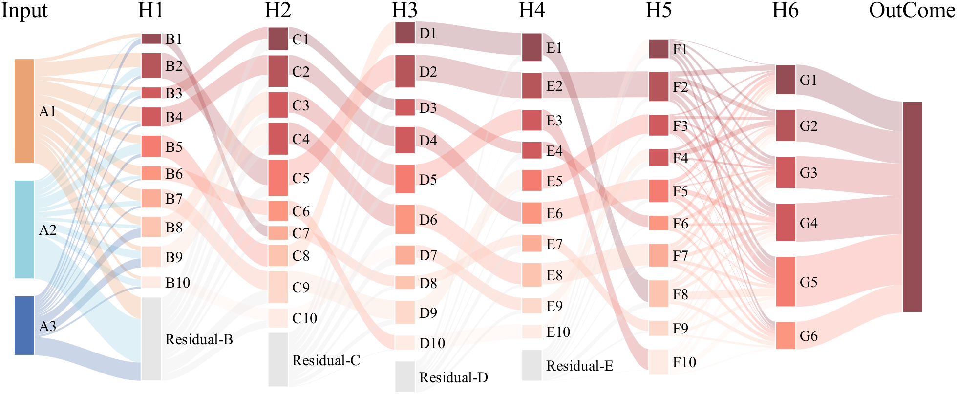
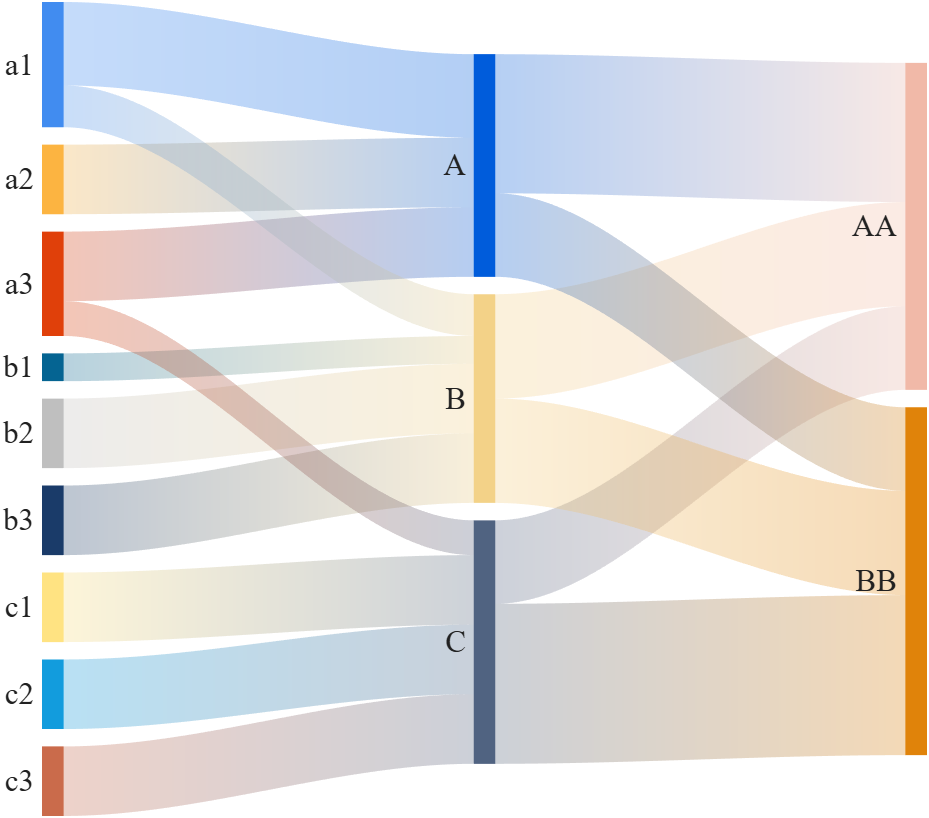
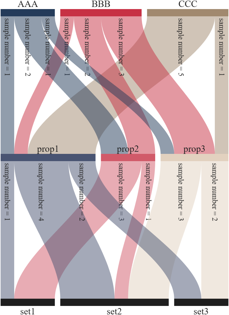
This is a brief introduction and recommendation of a Sankey diagram plotting tool:
Basic usage - links
links={'a1','A',1.2;'a2','A',1;'a1','B',.6;'a3','A',1; 'a3','C',0.5;
'b1','B',.4; 'b2','B',1;'b3','B',1; 'c1','C',1;
'c2','C',1; 'c3','C',1;'A','AA',2; 'A','BB',1.2;
'B','BB',1.5; 'B','AA',1.5; 'C','BB',2.3; 'C','AA',1.2};
% 创建桑基图对象(Create a Sankey diagram object)
SK=SSankey(links(:,1),links(:,2),links(:,3));
% 开始绘图(Start drawing)
SK.draw()
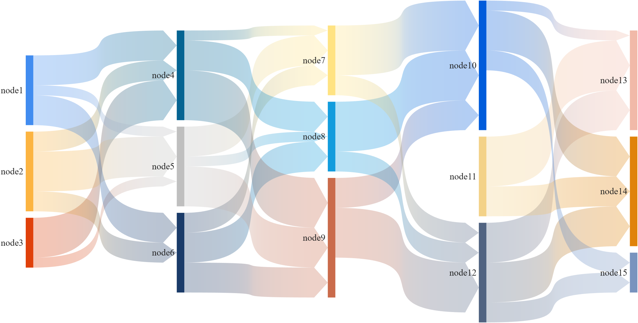
Basic usage - adjMat
% Define inter-layer adjacency matrices
% 定义层间邻接矩阵
A12 = [1,2,1; 1,2,3; 2,0,1];
A23 = [1,4; 2,1; 0,3];
A34 = [1,5; 2,3];
% Assemble global block matrix (main diagonal = zero, super-diagonal = A12, A23, A34)
% 组装全局分块矩阵(主对角线为零,上对角线为 A12, A23, A34)
adjMat = mergeAdjMat({A12, A23, A34});
SK = SSankey([],[],[], 'AdjMat',adjMat);
SK.draw()
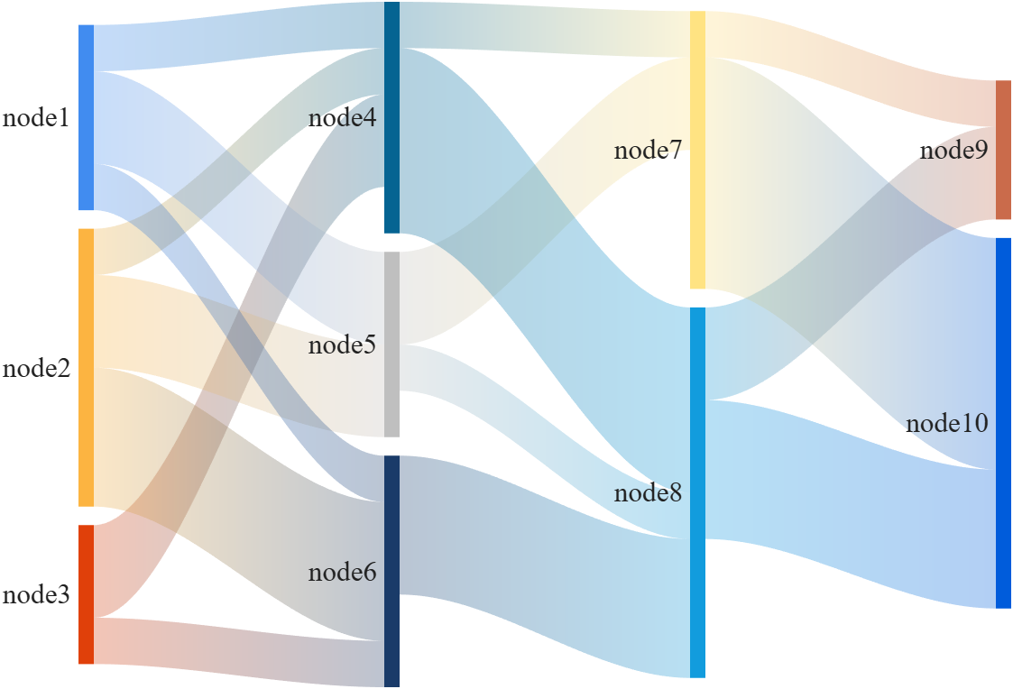
Further usage examples can be found in the demos included in the compressed package:
We’re excited to share that our new unified search experience is now live!
Anywhere you see the MATLAB Help Center | Community | Learning header, the search icon will now take you to the same results page. This makes it much easier to find content across different areas in one place—and you’ll also see an AI-powered response at the top to help you get quick answers.
A quick note: search from the homepage, product pages, solutions, and a few other areas will continue to work as they do today.
This update is all about making it easier to discover related content across the site, instead of being limited to one area at a time.
Give it a try and let us know what you think—we’d love your feedback!
I've been confused trying to write (or have an AI write) the .m (Live) text format from scratch for various reasons using .mlx format exported with the IDE as .m (old) and .m (LIve). Of course, one problem is the .m and .m (Live) files have the same name,causing confusion and requiring renaming, but repeatedly, after sussing out and following all conventions for headings and latex etc in .m (LIve), my .m (Live) files would not open as .mlx in the IDE. I think I've found the answer by trial and error and comparison and don't know it is documented. Add at the end
%[appendix]{"version":"1.0"} %--- %[metadata:view] % data: {"layout":"inline"} %---
This seems to trigger the IDE to recognize this is a .m (Live). Woohoo! This is a LOT easier than writing .mlx zip packages from scratch.

Generate a 3D visualization of carnation flowers
with sepals and stems for celebrating Mother's Day 2026.

function carnation
% CARNATION Generate a 3D visualization of carnation flowers with sepals and stems.
% This code is authored by Zhaoxu Liu / slandarer
% for the purpose of celebrating Mother's Day 2026.
% =========================================================================
% Zhaoxu Liu / slandarer (2026). carnation for Mother's Day
% (https://www.mathworks.com/matlabcentral/fileexchange/183838-carnation-for-mother-s-day),
% MATLAB Central File Exchange. Retrieved May 9, 2026.
% Create figure and axes / 创建图窗及坐标区域
fig = figure('Units','normalized', 'Position',[.3,.1,.4,.8],'Color',[244,234,225]./255);
axes('Parent',fig, 'NextPlot','add', 'DataAspectRatio',[1,1,1],...
'View',[-64, 5.5], 'Position',[0,-.15,1,1], 'Color',[244,234,225]./255, ...
'XColor','none', 'YColor','none', 'ZColor','none');
annotation("textbox", [.05, .8, .9, .2], "String", {"Happy"; "Mother's Day"}, ...
'FontName','Segoe Script', 'FontSize',52, 'FontWeight','bold', 'EdgeColor','none', ...
'HorizontalAlignment','center', 'VerticalAlignment','middle', 'Color',[97,40,20]./255);
xx = linspace(0, 1, 100);
tt = linspace(0, 1, 1e4);
[X, P] = meshgrid(xx, tt);
T1 = P*20*pi;
C1 = 1 - (1 - mod(3.6*T1/pi, 2)).^4./2; % Petal profile / 花瓣形状
S1 = (sin(50*T1)/150 + sin(10*T1)/30).*min(1, max(0, (X - .85)/.1)); % Edge serration / 边缘褶皱和锯齿
Y1 = (- (X.*1.2 - .5).^5.*32 - 1)./15.*P; % Petal curvature / 花瓣弧度
% Petal shape and serration modeling + rotating the planar petal to tilt it
% 花瓣形状和锯齿塑造 + 转动平躺的花瓣令其倾斜
R1 = (C1 + S1).*(X.*sin(P) - Y1.*cos(P))./(P + .5);
H1 = (C1 + S1).*(X.*cos(P) + Y1.*sin(P));
% Convert radius to Cartesian coordinates / 将半径映射为X,Y坐标
X1 = R1.*cos(T1);
Y1 = R1.*sin(T1);
% Colormap for carnation petals / 康乃馨配色
CList1 = [208, 62, 23; 221,146,121; 229,201,202; 233,219,222; 237,223,225]./255;
CMat1 = zeros(1e4, 100, 3);
CMat1(:, :, 1) = repmat(interp1(linspace(0, 1, size(CList1, 1)), CList1(:, 1), linspace(0, 1, 100)), [1e4, 1]);
CMat1(:, :, 2) = repmat(interp1(linspace(0, 1, size(CList1, 1)), CList1(:, 2), linspace(0, 1, 100)), [1e4, 1]);
CMat1(:, :, 3) = repmat(interp1(linspace(0, 1, size(CList1, 1)), CList1(:, 3), linspace(0, 1, 100)), [1e4, 1]);
% Darken edges / 边缘的深色
for i = 1:1e4
tNum = randi([98, 100]);
CMat1(i, tNum:end, 1) = 212./255;
CMat1(i, tNum:end, 2) = 87./255;
CMat1(i, tNum:end, 3) = 113./255;
end
% Rotation matrices / 旋转矩阵
Rx = @(rx) [1, 0, 0; 0, cos(rx), -sin(rx); 0, sin(rx), cos(rx)];
Rz = @(yz) [cos(yz), - sin(yz), 0; sin(yz), cos(yz), 0; 0, 0, 1];
Rx1 = Rx(pi/6); Rz1 = Rz(0);
% Render flower / 绘制康乃馨
surface(X1, Y1, H1 + .3, 'CData',CMat1, 'EdgeAlpha',0.1, 'EdgeColor',[224,39,39]./255, 'FaceColor','interp')
[U1, V1, W1] = matRotate(X1, Y1, H1 + .3, Rx1);
surface(U1 + .7, V1 - .7, W1 - .6, 'CData',CMat1, 'EdgeAlpha',0.1, 'EdgeColor',[224,39,39]./255, 'FaceColor','interp')
% Following the same method as before,
% the profile is designed with four serrated cycles to simulate the four sepals.
% 还是之前的方法,不过让轮廓有4个锯齿状周期来模拟四片花萼
% Sepals generation with 4-lobed pattern / 生成四片花萼(带4个锯齿状周期)
[X, T] = meshgrid(linspace(0, 1, 100), linspace(0, 1, 100).*2*pi);
P2 = T.*0 + pi/8;
C2 = .5 + (.5 - abs(mod(T, pi/2)/pi*2 - .5))*.4;
Y2 = (- (X.*1 - .5).^7.*128 - 1)./15 - .1;
R2 = C2.*(X.*sin(P2) - Y2.*cos(P2));
H2 = C2.*(X.*cos(P2) + Y2.*sin(P2));
X2 = R2.*cos(T);
Y2 = R2.*sin(T);
% Rotate by 90 degrees around the z-axis
% and reduce the size to render the four smaller sepals.
% 绕z轴旋转90度且减小其大小,绘制四片小花萼
% Smaller sepal layer / 绘制四片小花萼(第二层)
P3 = T.*0 + pi/10;
C3 = .3 + (.5 - abs(mod(T + pi/4, pi/2)/pi*2 - .5))*.7;
Y3 = (- (X.*.7 - .5).^7.*128 - 1)./15 - .1;
R3 = C3.*(X.*sin(P3) - Y3.*cos(P3));
H3 = C3.*(X.*cos(P3) + Y3.*sin(P3));
X3 = R3.*cos(T);
Y3 = R3.*sin(T);
% Colormap for sepals / 花托配色
CList2 = [178,173,113; 151,135, 73; 117,123, 50; 86, 89, 29; 75, 65, 17]./255;
CMat2 = zeros(100, 100, 3);
CMat2(:, :, 1) = repmat(interp1(linspace(0, 1, size(CList2, 1)), CList2(:, 1), linspace(0, 1, 100)), [100, 1]);
CMat2(:, :, 2) = repmat(interp1(linspace(0, 1, size(CList2, 1)), CList2(:, 2), linspace(0, 1, 100)), [100, 1]);
CMat2(:, :, 3) = repmat(interp1(linspace(0, 1, size(CList2, 1)), CList2(:, 3), linspace(0, 1, 100)), [100, 1]);
% Render sepals / 绘制花托
surf(X2, Y2, H2.*.8 + .12, 'CData',CMat2, 'EdgeAlpha',0.1, 'EdgeColor',CList2(end,:), 'FaceColor','interp')
surf(X3.*.93, Y3.*.92, H3.*.5 + .02, 'FaceColor',[ 84, 85, 54]./255, 'EdgeAlpha',0.1, 'EdgeColor','k')
[U2, V2, W2] = matRotate(X2, Y2, H2.*.8 + .12, Rx1);
[U3, V3, W3] = matRotate(X3.*.93, Y3.*.92, H3.*.5 + .02, Rx1);
surf(U2 + .7, V2 - .7, W2 - .6, 'CData',CMat2, 'EdgeAlpha',0.1, 'EdgeColor',CList2(end,:), 'FaceColor','interp')
surf(U3 + .7, V3 - .7, W3 - .6, 'FaceColor',[ 84, 85, 54]./255, 'EdgeAlpha',0.1, 'EdgeColor','k')
% A pulse function with two periods is applied
% to the contour to simulate the leaves.
% 让轮廓有2个周期且是脉冲函数,来模拟叶片
P4 = T.*0 + pi/16;
C4 = - abs(mod(T, pi)/pi - .5) + .11;
C4(C4 < 0) = 0; C4 = C4.*10; C4(51:100, :) = C4(51:100, :).*.7;
Y4 = (- (X.*1.01 - .5).^7.*128 - 1)./15 - .03;
R4 = C4.*(X.*sin(P4) - Y4.*cos(P4));
H4 = C4.*(X.*cos(P4) + Y4.*sin(P4));
X4 = R4.*cos(T);
Y4 = R4.*sin(T);
surf(X4 - .1, Y4 + .05, H4 - 2.2, 'FaceColor',[ 84, 85, 54]./255, 'EdgeAlpha',0.1, 'EdgeColor','k')
[U4, V4, W4] = matRotate(X4 - .1, Y4 - .1, H4 + .1, Rz1);
[U4, V4, W4] = matRotate(U4, V4, W4, Rx1);
surf(U4 + .7, V4 - .7 + 1, W4 - .6 - 1.2, 'FaceColor',[ 84, 85, 54]./255, 'EdgeAlpha',0.1, 'EdgeColor','k')
P5 = T.*0 + pi/8;
C5 = - abs(mod(T + pi/6, pi)/pi - .5) + .11;
C5(C5 < 0) = 0; C5 = C5.*5;
Y5 = (- (X.*1.01 - .5).^7.*128 - 1)./15 - .1;
R5 = C5.*(X.*sin(P5) - Y5.*cos(P5));
H5 = C5.*(X.*cos(P5) + Y5.*sin(P5));
X5 = R5.*cos(T);
Y5 = R5.*sin(T);
surf(X5, Y5, H5 - .3, 'FaceColor',[ 84, 85, 54]./255, 'EdgeAlpha',0.1, 'EdgeColor','k')
[U5, V5, W5] = matRotate(X5, Y5, H5+.1, Rx1);
surf(U5 + .7, V5 - .7 + 1/4, W5 - .6 - 1.7/4, 'FaceColor',[ 84, 85, 54]./255, 'EdgeAlpha',0.1, 'EdgeColor','k')
% Render stems / 绘制花杆
P1_1 = [mean(X3(:).*.93), mean(Y3(:).*.92), mean(H3(:).*.5 + .02)];
P1_2 = [mean(X5(:)), mean(Y5(:)), mean(H5(:) - .3)];
P1_3 = [mean(X4(:) - .1), mean(Y4(:) + .05), mean(H4(:) - 2.2)];
P1_3 = (P1_3 - P1_2).*1.4 + P1_2;
[XX1, YY1, ZZ1] = cylinderXYZ(P1_1, P1_2, .05);
[XX2, YY2, ZZ2] = cylinderXYZ(P1_2, P1_3, .04);
surf(XX1, YY1, ZZ1, 'FaceColor',[ 84, 85, 54]./255, 'EdgeAlpha',0.1, 'EdgeColor','k')
surf(XX2, YY2, ZZ2, 'FaceColor',[ 84, 85, 54]./255, 'EdgeAlpha',0.1, 'EdgeColor','k')
P1_1 = [mean(U3(:) + .7), mean(V3(:) - .7), mean(W3(:) - .6)];
P1_2 = [mean(U5(:) + .7), mean(V5(:) - .7 + 1/4), mean(W5(:) - .6 - 1.7/4)];
P1_3 = [mean(U4(:) + .7), mean(V4(:) - .7 + 1), mean(W4(:) - .6 - 1.2)];
P1_3 = (P1_3 - P1_2).*2.4 + P1_2;
[XX1, YY1, ZZ1] = cylinderXYZ(P1_1, P1_2, .05);
[XX2, YY2, ZZ2] = cylinderXYZ(P1_2, P1_3, .04);
surf(XX1, YY1, ZZ1, 'FaceColor',[ 84, 85, 54]./255, 'EdgeAlpha',0.1, 'EdgeColor','k')
surf(XX2, YY2, ZZ2, 'FaceColor',[ 84, 85, 54]./255, 'EdgeAlpha',0.1, 'EdgeColor','k')
% 在任意两点间构建圆柱
function [XX, YY, ZZ] = cylinderXYZ(P1, P2, r)
% CYLINDERXYZ Create a cylinder connecting two 3D points
% [XX, YY, ZZ] = cylinderXYZ(P1, P2, r) generates a cylinder
% of radius r between points P1 and P2.
v = P2 - P1; l = norm(v);
if l < eps, return; end
[XX, YY, ZZ] = cylinder(r, 30); ZZ = ZZ * l;
ddir = [0, 0, 1]; tdir = v / l;
if dot(ddir, tdir) > 0.9999
R = eye(3);
elseif dot(ddir, tdir) < -0.9999
R = [1, 0, 0; 0, -1, 0; 0, 0, -1];
else
av = cross(ddir, tdir); av = av / norm(av);
R = axisRotate(av, acos(dot(ddir, tdir)));
end
for ii = 1:size(XX, 1)
for jj = 1:size(XX, 2)
p = R * [XX(ii, jj); YY(ii, jj); ZZ(ii, jj)];
XX(ii, jj) = p(1) + P1(1);
YY(ii, jj) = p(2) + P1(2);
ZZ(ii, jj) = p(3) + P1(3);
end
end
end
% 通过矩阵旋转数据
function [U, V, W] = matRotate(X, Y, Z, R)
% MATROTATE Apply 3x3 rotation matrix to a set of 3D points
% [U,V,W] = matRotate(X,Y,Z,R) rotates points (X,Y,Z)
% using rotation matrix R.
U = X; V = Y; W = Z;
for ii = 1:numel(X)
v = [X(ii); Y(ii); Z(ii)];
n = R*v; U(ii) = n(1); V(ii) = n(2); W(ii) = n(3);
end
end
% 根据轴-角参数生成旋转矩阵
function R = axisRotate(axis, angle)
% AXISROTATE Compute rotation matrix from axis-angle representation
% R = axisRotate(axis, angle) returns a 3x3 rotation matrix
% for rotating by angle (radians) around the given axis vector.
% Implementation based on Rodrigues' rotation formula.
u = axis(1); v = axis(2); w = axis(3);
c = cos(angle); s = sin(angle);
R = [u^2 + (1-u^2)*c, u*v*(1-c) - w*s, u*w*(1-c) + v*s;
u*v*(1-c) + w*s, v^2 + (1-v^2)*c, v*w*(1-c) - u*s;
u*w*(1-c) - v*s, v*w*(1-c) + u*s, w^2 + (1-w^2)*c];
end
end
We’re excited to share that Cleve Moler, creator of MATLAB, has been elected to the U.S. National Academy of Sciences—one of the highest honors in science.
This recognition celebrates Cleve’s groundbreaking contributions to numerical computing and his lasting impact on researchers, educators, and engineers around the world. From advancing numerical linear algebra to making powerful computation more accessible through MATLAB, his work has shaped how science and engineering are done today.
Please join us in congratulating Cleve on this well‑deserved honor!
🔗 Learn more about the 2026 NAS election
Hello Community,
Registration is now open for the MathWorks Automotive Conference 2026 North America. Join industry leaders and MathWorks experts to learn about the latest trends in:
- Software-defined vehicles
- Generative AI
- Virtual vehicles
- AI and machine learning
Event details
- Date: April 28, 2026
- Location: Saint John’s Resort, Plymouth, MI
This conference is a great opportunity to connect with MathWorks and industry peers—and to explore what’s next in automotive engineering. We encourage you to register today.
We hope to see you there.
Have you ever wondered what it takes to send live audio from one computer to another? While we use apps like Discord and Zoom every day, the core technology behind real-time voice communication is a fascinating blend of audio processing and networking. Building a simple walkie-talkie is a perfect project for demystifying these concepts, and you can do it all within the powerful environment of MATLAB.
This article will guide you through creating a functional, real-time, push-to-talk walkie-talkie. We won't be building a replacement for a commercial radio, but we will create a powerful educational tool that demonstrates the fundamentals of digital signal processing and network communication.
The Purpose: Why Build This?
The goal isn't just to talk to a colleague across the office; it's to learn by doing. By building this project, you will:
Understand Audio I/O: Learn how MATLAB interacts with your computer’s microphone and speakers.
Grasp Network Communication: See how to send data packets over a local network using the UDP protocol.
Solve Real-Time Challenges: Confront and solve issues like latency, choppy audio, and continuous data streaming.
The Core Components
Our walkie-talkie will consist of two main scripts:
Sender.m: This script will run on the transmitting computer. It listens to the microphone when a key is pressed, sending the audio data in small chunks over the network.
Receiver.m: This script runs on the receiving computer. It continuously listens for incoming data packets and plays them through the speakers as they arrive.
Step 1: Getting Audio In and Out
Before we touch networking, let's make sure we can capture and play audio. MATLAB's built-in audiorecorder and audioplayer objects make this simple.
Problem Encountered: How do you even access the microphone?
Solution: The audiorecorder object gives us straightforward control.
code
% --- Test Audio Capture and Playback ---
Fs = 8000; % Sample rate in Hz
nBits = 16; % Number of bits per sample
nChannels = 1; % Mono audio
% Create a recorder object
recObj = audiorecorder(Fs, nBits, nChannels);
disp('Start speaking for 3 seconds.');
recordblocking(recObj, 3); % Record for 3 seconds
disp('End of Recording.');
% Get the audio data
audioData = getaudiodata(recObj);
% Play it back
playObj = audioplayer(audioData, Fs);
play(playObj);
Running this script confirms that your microphone and speakers are correctly configured and accessible by MATLAB.
Step 2: Sending Voice Over the Network
Now, we need to send the audioData to another computer. For real-time applications like this, the UDP (User Datagram Protocol) is the ideal choice. It’s a "fire-and-forget" protocol that prioritizes speed over perfect reliability. Losing a tiny packet of audio is better than waiting for it to be re-sent, which would cause noticeable delays (latency).
Problem Encountered: How do you send data continuously without overwhelming the network or the receiver?
Solution: We'll send the audio in small, manageable chunks inside a loop. We need to create a UDP Port object to handle the communication.
Here's the basic structure for the Sender.m script:
code
% --- Sender.m ---
% Define network parameters
remoteIP = '192.168.1.101'; % <--- CHANGE THIS to the receiver's IP
remotePort = 3000;
localPort = 3001;
% Create UDP Port object
udpSender = udpport("LocalPort", localPort, "EnablePortSharing", true);
% Configure audio recorder
Fs = 8000;
nBits = 16;
nChannels = 1;
recObj = audiorecorder(Fs, nBits, nChannels);
disp('Press any key to start transmitting. Press Ctrl+C to stop.');
pause; % Wait for user to press a key
% Start the Push-to-Talk loop
disp('Transmitting... (Hold Ctrl+C to exit)');
while true
recordblocking(recObj, 0.1); % Record a 0.1-second chunk
audioChunk = getaudiodata(recObj);
% Send the audio chunk over UDP
write(udpSender, audioChunk, "double", remoteIP, remotePort);
end
And here is the corresponding Receiver.m script:
code
Matlab
% --- Receiver.m ---
% Define network parameters
localPort = 3000;
% Create UDP Port object
udpReceiver = udpport("LocalPort", localPort, "EnablePortSharing", true, "Timeout", 30);
% Configure audio player
Fs = 8000;
playerObj = audioplayer(zeros(Fs*0.1, 1), Fs); % Pre-buffer
disp('Listening for incoming audio...');
% Start the listening loop
while true
% Wait for and receive data
[audioChunk, ~, ~] = read(udpReceiver, Fs*0.1, "double");
if ~isempty(audioChunk)
% Play the received audio chunk
play(playerObj, audioChunk);
else
disp('No data received. Still listening...');
end
end
Step 3: Solving Real-World Hurdles
Running the code above might work, but you'll quickly notice some issues.
Problem 1: Choppy Audio and High Latency
The audio might sound robotic or delayed. This is because of the buffer size and the processing time. Sending tiny chunks frequently can cause overhead, while sending large chunks causes delay.
Solution: The key is to find a balance.
Tune the Chunk Size: The 0.1 second chunk size in the sender (recordblocking(recObj, 0.1)) is a good starting point. Experiment with values between 0.05 and 0.2. Smaller values reduce latency but increase network traffic.
Use a Buffered Player: Instead of creating a new audioplayer for every chunk, we create one at the start and feed it new data. Our receiver code already does this, which is more efficient.
Problem 2: No Real "Push-to-Talk"
Our sender script starts transmitting and doesn't stop. A real walkie-talkie only transmits when a button is held down.
Solution: Simulating this in a script requires a more advanced technique, ideally using a MATLAB App Designer GUI. However, we can create a simple command-window version using a figure's KeyPressFcn.
Here is an improved concept for the Sender that simulates radio push-to-talk, e.g. https://www.retevis.com/blog/ptt-push-to-talk-walkie-talkies-guide
% --- Advanced_Sender.m ---
function PushToTalkSender()
% -- Configuration --
remoteIP = '192.168.1.101'; % <--- CHANGE THIS
remotePort = 3000;
localPort = 3001;
Fs = 8000;
% -- Setup --
udpSender = udpport("LocalPort", localPort);
recObj = audiorecorder(Fs, 16, 1);
% -- GUI for key press detection --
fig = uifigure('Name', 'Push-to-Talk (Hold ''t'')', 'Position', [100 100 300 100]);
fig.KeyPressFcn = @KeyPress;
fig.KeyReleaseFcn = @KeyRelease;
isTransmitting = false; % Flag to control transmission
disp('Focus on the figure window. Hold the ''t'' key to transmit.');
% --- Main Loop ---
while ishandle(fig)
if isTransmitting
% Non-blocking record and send would be ideal,
% but for simplicity we use short blocking chunks.
recordblocking(recObj, 0.1);
audioChunk = getaudiodata(recObj);
write(udpSender, audioChunk, "double", remoteIP, remotePort);
disp('Transmitting...');
else
pause(0.1); % Don't burn CPU when idle
end
drawnow; % Update figure window
end
% --- Callback Functions ---
function KeyPress(~, event)
if strcmp(event.Key, 't')
isTransmitting = true;
end
end
function KeyRelease(~, event)
if strcmp(event.Key, 't')
isTransmitting = false;
disp('Transmission stopped.');
end
end
end
Conclusion and Next Steps
You've now built the foundation of a real-time voice communication tool in MATLAB! You've learned how to capture audio, send it over a network using UDP, and handle some of the fundamental challenges of real-time streaming.
This project is the perfect starting point for more advanced explorations:
Build a Full GUI: Use App Designer to create a user-friendly interface with a proper push-to-talk radio button.
Implement Noise Reduction: Apply a filter (e.g., a simple low-pass or a more advanced spectral subtraction algorithm) to the audioChunk before sending it.
Add Channels: Modify the code to use different UDP ports, allowing users to select a "channel" to talk on.
In a previous discussion,
we looked at a variety of infallible tests for primality, but all of them were too slow to be viable for large numbers. In fact, all of the methods discussed there will fail miserably for even moderately large numbers, those with just a few dozen decimal digits. That does not even begin to push into the realm of large numbers. In turn, that forces us into a different realm of tests - tests which are usually and even almost always correct, but can sometimes incorrectly predict primality.
In this discussion, I will be trying to convince you that the Fermat test for primality can be a quite good test when the number is sufficiently large. Except of course, when it is really bad. Even so, the Fermat test for primality is both a useful tool as well as a necessary underpinning for several other better tests.
The Fermat test for primality relies on Fermat's little theorem, a perhaps under-appreciated tool. Even the name implies it is of little interest. I'm not taking about the famous last theorem, only proven in recent years, but his little theorem.
If you want to look over some nice ways to prove the little theorem, take a read in this link:
I will readily admit that long ago, when I learned about the little theorem in a nearly forgotten class, I thought it was interesting, but why would I care? Not until I learned more mathematics and saw Fermat’s little theorem appearing in different places did I begin to appreciate it. Fermat tells us that, IF P is a prime, AND w is co-prime with P (so the two are relatively prime, sharing no common factors except 1), then it must be true that
mod(w^(P-1),P) == 1
Try it out. Does it work? Be careful though as too large of an exponent will cause problems in double precision, and that is not difficult to do. As a test case that will not overwhelm doubles, note that 13 is prime, and 3 shares no common factors with 13, so we satisfy the requirements for Fermat's little theorem.
mod(3^12,13)
We can even verify that any co-prime of 13 will yield the same result.
mod((1:12).^12,13)
Indeed it worked, suggesting what we knew all along, that 13 is prime. The little Fermat test for primality of the number P uses a converse form of Fermat's little theorem, thus given a co-prime number w known as the witness, is that if
mod(w^(P-1),P)==1
then we have evidence that P is indeed prime. This is not conclusive evidence, but still it is evidence. It is not conclusive because the converse of a true statement is not always true.
The analogy I like here is if we lived in a universe where all crows are black. (I'll ask you to pretend this is true. In fact, some crows have a mutation, making them essentially albino crows. For the purposes of this thought experiment, pretend this cannot happen.) Now, suppose I show you a picture of a bird which happens to be black. Do you know the bird to be a crow? Of course not, as the bird may be a raven, or a redwing blackbird (until you see the splash of red on the wing), a common grackle, a European starling in summer plumage, a condor, etc. But having seen black plumage, it is now more likely the bird is indeed a crow. I would call this a moderately weak evidentiary test for crow-ness.
Little Fermat may seem to be of little value when testing for primality for two reasons. First, computing the remainder would seem to be highly CPU intensive for large P. In the example above, I had only to compute 3^12=531441, which is not that large. But for numbers with many thousands or millions of digits, directly raising even a number as small as 2 to that power will overwhelm any computer. Secondly, if we do that computation, little Fermat does not conclusively prove P to be prime.
Our savior in one respect is the powermod tool. And that helps greatly, since we can compute the remainder in a reasonable time. A powermod call is quite fast even for huge powers. (I won't get into how powermod works here, since that alone is probably worth a discussion. I could though, if I see some interest because there are some very pretty variations of the powermod algorithm. I hope to show you one of them when I discuss the Fibonacci test for primality in a future post.) Trying the little Fermat test using powermod on a number with 1207 decimal digits, I’ll first do a time check.
P = 4000*sym(2)^3999 - 1;
timeit(@() powermod(2,P-1,P))
As you can see, powermod really is pretty fast. Compared to an isprime test on that number it would show a significant difference.
I have said before that little Fermat is not a conclusive test. In fact, a good trick is to perform a second little Fermat test, using a different witness. If the second test also indicates primality, then we have additional evidence that P is in fact prime.
w = [2 3]; % Two parallel witnesses
powermod(w,P-1,P)
This value for P is indeed prime, and little Fermat suggests it is, doubly suggestive in that test since I actually performed two parallel tests. Here however, we need to understand when it will fail, and how often it will fail.
If we perform a little Fermat test for primality, we will never see false negatives, that is, if any test with any witness ever indicates a number is composite, then it is certainly composite. (The contrapositive of a true statement is always true.) The alternate class of failure is the false positive, where little Fermat indicates a number is prime when it was actually composite.
If P is composite, and w co-prime with P, we call P a Fermat pseudo-prime for the witness w if we see a remainder of 1 when P was in fact composite. When that happens, the witness (w) is called a Fermat liar for the primality of P. (A list of some Fermat pseudo-primes where 2 is a Fermat liar can be found in sequence A001567 of the OEIS.)
In the case of 4000*2^3999-1, I claimed the number to be in fact prime, and it was identified so (as PROBABLY prime by little Fermat. Next, consider another number from that same family. I’ll perform three parallel tests on it, with witnesses 2, 3, and 5. This will suggest the value of doing parallel tests on a number to reduce the failure rate from little Fermat.
P2 = 1024*sym(2)^1023 - 1;
w = [2; 3; 5];
gcd(w,P2)
F2 = powermod(w,P2-1,P2)
logical(F2 == 1)
As you can see, P2 is co-prime with all of 2, 3 and 5, but 2 is a Fermat liar, whilst 3 and 5 are Fermat truth tellers, identifying P2 as certainly composite. So the little Fermat test can definitely fail for SOME witnesses, since we see a disagreement. However, an interesting fact about P2 above is it is also a Mersenne number with prime exponent, thus it can be written as 2^1033-1, where 1033 is prime. I can go into more detail about this case later, but we can show that 2 is always a Fermat liar for composite Mersenne numbers when the exponent is itself prime. I’ll try to leave more detail on this matter in a future discussion, or perhaps a comment.
Next, consider the composite integer 51=3*17. As the product of two primes, it is clearly not itself prime.
P51 = 51;
w0 = 2:P51-2;
w = w0(gcd(w0,P51) == 1)
Note that I did not include 1 or 50 in that set, since 1 raised to any power is 1, and 50 is congruent to -1, mod 51. -1 raised to any even power is also always 1, and 51-1 is an even number. And so when we are working modulo 51, both 1 and 50 are not useful witnesses in terms of the little Fermat test.
R = powermod(w,P-1,P)
w(R == 1)
This teaches us that when 51 is tested for primality using the little Fermat test, there are 2 distinct witnesses w (16 and 35) we could have chosen which would have been Fermat liars, but all 28 other potential co-prime witnesses would have been truth tellers, accurately showing 51 to be composite. Proportionally, little Fermat will have been correct roughly 93% of the time, since only 2 of these 30 possible tests returned a false positive. (I’ll add that for any modulus P, if w<P is not co-prime with the modulus, then the computation mod(w^(P-1),P) will always return a non-unit result, and therefore we can theoretically use any integer w from the set 2:P-2 as a witness. However if w is co-prime with P then P is clearly not prime, and the entire problem becomes a little less interesting. As such, I will only consider co-prime witnesses for this discussion.) Regardless, that would make the little Fermat test for P=51 even more often correct, since it returns the correct result of composite for 46 out of the 48 possible witnesses 2:49. Does this mean Little Fermat is indeed the basis for a good test to rely on to learn if a number is prime? Well, yes. And no.
Little Fermat forms a very good test most of the time, but reliance is a strong word. This means we need to explore the little Fermat test in more depth, focusing on Fermat liars and the case of false positives. To offer some appreciation of the false positive rate, offline, I have tested all composite integers between 4 and 10000, for all their possible co-prime witnesses.
load FermatLiarsData
In that .mat file, I've saved three vectors, X, witnessCount, and liarCount. X is there just to use for plotting purposes and is NaN for all non-composite entries.
whos X witnessCount liarCount
The vector witnessCount is the number of valid witnesses for the corresponding number in X. Corresponding to that is the vector liarCount, which is the number of Fermat liars I found for each composite in X.
How many Fermat test useful witnesses are there for any integer X? This is just 2 less than the number of coprimes of X. The number of coprimes is given by the Euler totient function, commonly called phi(X). (I’ll be going into more depth on the totient in the next chapter of this series, because the Euler totient is a crucial part of understanding how all of this works.)
The witness count is phi(X)-2. Why subtract 2? 1 can never be a witness, but 1 is technically coprime to everything. The same applies to X-1 (which is congruent to -1 mod X.) As such, there are phi(X)-2 coprimes to consider. (I've posted a function called totient on the FEX, but it is easily computed if you know the factorization of X. Or for small numbers, you can just use GCD to identify all co-primes, and count them.)
plot(X,witnessCount,'.')
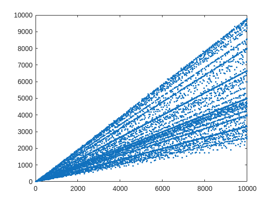
From that plot, you can learn a few interesting things. (As a mathematician, this is what I love the most, thus to look at whay may be the simplest, most boring plot, and try to find something of value, something I had never thought of before.) For example, we know that when X is prime, then everything from the set 2:X-2 is a valid witness. So the upper boundary on that plot will be the line y==x. As well, there are a few numbers where the order of the set of witnesses will be close to the maximum possible. For example, 961=31*31, has 928 valid witnesses. That makes some sense, as 961 is the square of a prime (31), so we know 961 is divisible only by 31. Only multiples of 31 will not be coprime with 961.
But how about the lower boundary? The least number of valid witnesses will always come from highly composite numbers, because they will share common factors with almost everything. For example 30 = 2*3*5, or 210=2*3*5*7.
witnessCount([30 210 420])
A good discussion about the lower bound for that plot can be found here:
What really matters to us though, is the fraction of the useful witnesses for a little Fermat test that yield a false positive.
plot(X,liarCount./witnessCount,'b.')
Cind = liarCount == witnessCount;
hold on
plot(X(Cind),1,'ro')
ylabel('Liar fraction')
xlabel('X')
title('Fermat pseudo-prime strength')
hold off
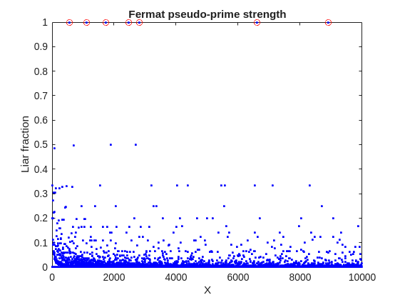
A look at this plot shows seven circles in red, corresponding to X from the list {561, 1105, 1729, 2465, 2821, 6601, 8911} which are collectively known as Carmichael numbers. These are numbers where all witnesses return a false positive. Carmichael numbers are themselves fairly rare. You can find a list of them as sequence A002997 in the OEIS. And for those of you who have never wandered around the OEIS, please take this opportunity to do so now. The OEIS stands for Online Encyclopedia of Integer Sequences. It contains a wealth of interesting knowledge about integers and integer sequences.)
There are a few other interesting numbers we can find in that plot, like 91 and 703, where roughly 50% of the valid witnesses yield false positives. Of the complete set, which numbers did return at least a 25% false positive rate for primality? These numbers would be known as strong pseudo-primes for the little Fermat test, because they are pseudo-primes for at least 25% of the potential witnesses. These strong pseudo-primes have some interesting similarities to the Carmichael numbers. (My next post will go into more depth on Carmichael numbers and strong pseudo-primes. At the moment, I am merely interested in looking at the how often the little Fermat test fails overall.)
find(liarCount./witnessCount> 0.25)
You should notice the spacing between successive strong Fermat pseudo-primes is growing slowly, with a spacing of roughly 800 on average in the vicinity of 10000. If I step out beyond by a factor of 10, the next strong Fermat pseudo-primes after 1e5 are {101101, 104653, 107185, 109061, 111361, 114589, 115921 126217, 126673}, so that average spacing is definitely growing.
Given that set, now we can look at the prime factorizations of each of those strong pseudo-primes. Can we learn something about them?
arrayfun(@factor,find(liarCount./witnessCount> 0.25),'UniformOutput',false)
Perhaps the most glaring thing I see in that set of factors is almost all of those strong Fermat pseudo-primes are square free. That is, in that list, only 45=3*3*5 had any replicated factor at all. That property of being square free is something we will see is necessary to be a Carmichael number, but it also suggests that a simple roughness test applied in advance would have eliminated almost all of those strong pseudo-primes as obviously not prime, even at a very low level of roughness.
In fact, for most composite integers, most witnesses do indeed return a negative, indicating the number is not prime, and therefore composite. Little Fermat does not commonly tell falsehoods, even though it can do so.
semilogy(X,movmedian(liarCount./witnessCount,20,'omitnan'),'b-')
title('False positive fraction for composites')
yline(0.0003,'r')

We can learn from this last plot that as the number to be tested grows large, the median false positive rate for little Fermat, even for X as low as only 10000, is roughly 0.0003. (It continues to decrease for larger X too. In fact, I’ve read that when X is on the order of 2^256, the relative fraction of Fermat liars is on the order of 1 in 1e12, and it continues to decrease as X grows in magnitude. In my eyes, that seems pretty good for an imperfect test. Not perfect, but not bad when paired with roughness and perhaps a second little Fermat test using a different witness, and we will start to see tests which bear a higher degree of strength.)
I’ll stop at this point in this post because the post is getting lengthy. In my next post, I’d like to visit some questions about what are Carmichael numbers, about whether some witnesses are better than others, and if there are any numbers which lack any Fermat liars. However, in order to dive more deeply, I will need to explain how/why/when the little Fermat test works, and what causes Fermat liars. Stay tuned, because this starts to get interesting.
Over the past few days I noticed a minor change on the MATLAB File Exchange:
For a FEX repository, if you click the 'Files' tab you now get a file-tree–style online manager layout with an 'Open in new tab' hyperlink near the top-left. This is very useful:
If you want to share that specific page externally (e.g., on GitHub), you can simply copy that hyperlink. For .mlx files it provides a perfect preview. I'd love to hear your thoughts.
EXAMPLE:
🤗🤗🤗
I recently created a short 5-minute video covering 10 tips for students learning MATLAB. I hope this helps!
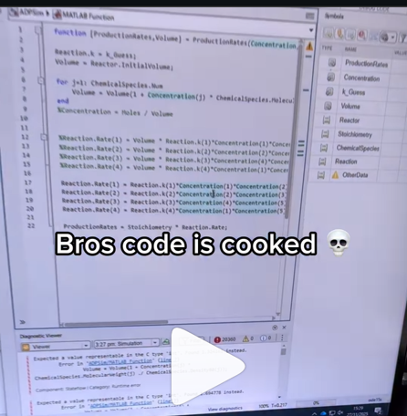
A coworker shared with me a hilarious Instagram post today. A brave bro posted a short video showing his MATLAB code… casually throwing 49,000 errors!
Surprisingly, the video went virial and recieved 250,000+ likes and 800+ comments. You really never know what the Instagram algorithm is thinking, but apparently “my code is absolutely cooked” is a universal developer experience 😂
Last note: Can someone please help this Bro fix his code?
In 2025, we saw the growing impact of GenAI on site traffic and user behavior across the entire technical landscape. Amid all this change, MATLAB Central continued to stand out as a trusted home for MATLAB and Simulink users. More than 11 million unique visitors in 2025 came to MATLAB Central to ask questions, share code, learn, and connect with one another.
Let’s celebrate what made 2025 memorable across three key areas: people, content, and events.
People
In 2025, nearly 20,000 contributors participated across the community. We’d like to spotlight a few standout contributors:
- @Sam Chak earned the Most Accepted Answers Badge for both 2024 and 2025. Sam is a rising star in MATLAB Answers with 2,000+ answers and 1,000+ votes.
- @Rodney Tan has been actively contributing files to File Exchange. In 2025, his submissions got almost 20,000 downloads!
- @Dyuman Joshi was recognized as a top contributor on both Cody and Answers. Many may not know that Dyuman is also a Cody moderator, doing tremendous behind-the-scenes moderation work to keep the platform running smoothly.
- A warm welcome to @Steve Eddins, who joined the Community Advisory Board. Steve brings a unique perspective as a former MathWorker and long-time top community contributor.
- Congratulations to @Walter Roberson on reaching 100 followers! MATLAB Central thrives on people-to-people connections, and we’d love to see even more of these relationships grow.
Of course, there are many contributors we didn’t mention here—thank you all for your outstanding contributions and for making the community what it is.
Content
Our high-quality community content not only attracts users but also helps power the broader GenAI ecosystem.
Popular Blog Post & File Exchange Submission
- Zoomed Axes, submitted by @Caleb Thomas, enables zoomed-in views of selected regions in a plot.This submission was featured in the Pick of the Week blog post, “MATLAB Zoomed Axes: Showing zoomed-in regions of a 2D plot,” which generated 5,000 views in just one month.
Popular Discussion Post
- What did MATLAB/Simulink users wait for most in 2025? It's R2025a! “Where is MATLAB R2025a?” became the most-viewed discussion post, with 10,000 views and 30 comments. Thanks for your patience — MATLAB R2025a turned out to be one of the biggest releases we’ve ever delivered.
Most Viewed Question
- “How do I create a for loop in MATLAB?” was the most-viewed community question of the year. It’s a fun reminder that even as MATLAB evolves, the basics remain essential — and always in demand.
Most Voted Poll
- “Did you know there is an official MATLAB certification?”, created by @goc3, was the most-voted poll of 2025.While 50% of respondents voted “No”, it’s exciting to see 3% are certified MATLAB Professionals. Will you be one of them in 2026?
Events
The Cody Contest 2025 brought teams together to tackle challenging but fun Cody problems. During the contest:
- 20,000+ solutions were submitted
- 20+ tips & tricks articles were shared by top players
While the contest has ended, you can still challenge yourself with the fun contest problem group. If you get stuck, the tips & tricks articles are a great resource—and you’ll be amazed by the creativity and skill of the contributors.
Thank you for being part of an incredible 2025. Your curiosity, generosity, and expertise are what make MATLAB Central a trusted home for millions—and we look forward to learning and growing together in 2026.
You may have come across code that looks like that in some languages:
stubFor(get(urlPathEqualTo("/quotes"))
.withHeader("Accept", equalTo("application/json"))
.withQueryParam("s", equalTo(monitoredStock))
.willReturn(aResponse())
.withStatus(200)
.withHeader("Content-Type", "application/json")
.withBody("{\\"symbol\\": \\"XYZ\\", \\"bid\\": 20.2, " + "\\"ask\\": 20.6}")))
That’s Java. Even if you can’t fully decipher it, you can get a rough idea of what it is supposed to do, build a rather complex API query.
Or you may be familiar with the following similar and frequent syntax in Python:
import seaborn as sns
sns.load_dataset('tips').sample(10, random_state=42).groupby('day').mean()
Here’s is how it works: multiple method calls are linked together in a single statement, spanning over one or several lines, usually because each method returns the same object or another object that supports further calls.
That technique is called method chaining and is popular in Object-Oriented Programming.
A few years ago, I looked for a way to write code like that in MATLAB too. And the answer is that it can be done in MATLAB as well, whevener you write your own class!
Implementing a method that can be chained is simply a matter of writing a method that returns the object itself.
In this article, I would like to show how to do it and what we can gain from such a syntax.
Example
A few years ago, I first sought how to implement that technique for a simulation launcher that had lots of parameters (far too many):
lauchSimulation(2014:2020, true, 'template', 'TmplProd', 'Priority', '+1', 'Memory', '+6000')
As you can see, that function takes 2 required inputs, and 3 named parameters (whose names aren’t even consistent, with ‘Priority’ and ‘Memory’ starting with an uppercase letter when ‘template’ doesn’t).
(The original function had many more parameters that I omit for the sake of brevity. You may also know of such functions in your own code that take a dozen parameters which you can remember the exact order.)
I thought it would be nice to replace that with:
SimulationLauncher() ...
.onYears(2014:2020) ...
.onDistributedCluster() ... % = equivalent of the previous "true"
.withTemplate('TmplProd') ...
.withPriority('+1') ...
.withReservedMemory('+6000') ...
.launch();
The first 6 lines create an object of class SimulationLauncher, calls several methods on that object to set the parameters, and lastly the method launch() is called, when all desired parameters have been set.
To make it cleared, the syntax previously shown could also be rewritten as:
launcher = SimulationLauncher();
launcher = launcher.onYears(2014:2020);
launcher = launcher.onDistributedCluster();
launcher = launcher.withTemplate('TmplProd');
launcher = launcher.withPriority('+1');
launcher = launcher.withReservedMemory('+6000');
launcher.launch();
Before we dive into how to implement that code, let’s examine the advantages and drawbacks of that syntax.
Benefits and drawbacks
Because I have extended the chained methods over several lines, it makes it easier to comment out or uncomment any one desired option, should the need arise. Furthermore, we need not bother any more with the order in which we set the parameters, whereas the usual syntax required that we memorize or check the documentation carefully for the order of the inputs.
More generally, chaining methods has the following benefits and a few drawbacks:
Benefits:
- Conciseness: Code becomes shorter and easier to write, by reducing visual noise compared to repeating the object name.
- Readability: Chained methods create a fluent, human-readable structure that makes intent clear.
- Reduced Temporary Variables: There's no need to create intermediary variables, as the methods directly operate on the object.
Drawbacks:
- Debugging Difficulty: If one method in a chain fails, it can be harder to isolate the issue. It effectively prevents setting breakpoints, inspecting intermediate values, and identifying which method failed.
- Readability Issues: Overly long and dense method chains can become hard to follow, reducing clarity.
- Side Effects: Methods that modify objects in place can lead to unintended side effects when used in long chains.
Implementation
In the SimulationLauncher class, the method lauch performs the main operation, while the other methods just serve as parameter setters. They take the object as input and return the object itself, after modifying it, so that other methods can be chained.
classdef SimulationLauncher
properties (GetAccess = private, SetAccess = private)
years_
isDistributed_ = false;
template_ = 'TestTemplate';
priority_ = '+2';
memory_ = '+5000';
end
methods
function varargout = launch(obj)
% perform whatever needs to be launched
% using the values of the properties stored in the object:
% obj.years_
% obj.template_
% etc.
end
function obj = onYears(obj, years)
assert(isnumeric(years))
obj.years_ = years;
end
function obj = onDistributedCluster(obj)
obj.isDistributed_ = true;
end
function obj = withTemplate(obj, template)
obj.template_ = template;
end
function obj = withPriority(obj, priority)
obj.priority_ = priority;
end
function obj = withMemory( obj, memory)
obj.memory_ = memory;
end
end
end
As you can see, each method can be in charge of verifying the correctness of its input, independantly. And what they do is just store the value of parameter inside the object. The class can define default values in the properties block.
You can configure different launchers from the same initial object, such as:
launcher = SimulationLauncher();
launcher = launcher.onYears(2014:2020);
launcher1 = launcher ...
.onDistributedCluster() ...
.withReservedMemory('+6000');
launcher2 = launcher ...
.withTemplate('TmplProd') ...
.withPriority('+1') ...
.withReservedMemory('+7000');
If you call the same method several times, only the last recorded value of the parameter will be taken into acount:
launcher = SimulationLauncher();
launcher = launcher ...
.withReservedMemory('+6000') ...
.onDistributedCluster() ...
.onYears(2014:2020) ...
.withReservedMemory('+7000') ...
.withReservedMemory('+8000');
% The value of "memory" will be '+8000'.
If the logic is still not clear to you, I advise you play a bit with the debugger to better understand what’s going on!
Conclusion
I love how the method chaining technique hides the minute detail that we don’t want to bother with when trying to understand what a piece of code does.
I hope this simple example has shown you how to apply it to write and organise your code in a more readable and convenient way.
Let me know if you have other questions, comments or suggestions. I may post other examples of that technique for other useful uses that I encountered in my experience.
If you use tables extensively to perform data analysis, you may at some point have wanted to add new functionalities suited to your specific applications. One straightforward idea is to create a new class that subclasses the built-in table class. You would then benefit from all inherited existing methods.
One workaround is to create a new class that wraps a table as a Property, and re-implement all the methods that you need and are already defined for table. The is not too difficult, except for the subsref method, for which I’ll provide the code below.
Class definition
Defining a wrapper of the table class is quite straightforward. In this example, I call the class “Report” because that is what I intend to use the class for, to compute and store reports. The constructor just takes a table as input:
classdef Rapport
methods
function obj = Report(t)
if isa(t, 'Report')
obj = t;
else
obj.t_ = t;
end
end
end
properties (GetAccess = private, SetAccess = private)
t_ table = table();
end
end
I designed the constructor so that it converts a table into a Report object, but also so that if we accidentally provide it with a Report object instead of a table, it will not generate an error.
Reproducing the behaviour of the table class
Implementing the existing methods of the table class for the Report class if pretty easy in most cases.
I made use of a method called “table” in order to be able to get the data back in table format instead of a Report, instead of accessing the property t_ of the object. That method can also be useful whenever you wish to use the methods or functions already existing for tables (such as writetable, rowfun, groupsummary…).
classdef Rapport
...
methods
function t = table(obj)
t = obj.t_;
end
function r = eq(obj1,obj2)
r = isequaln(table(obj1), table(obj2));
end
function ind = size(obj, varargin)
ind = size(table(obj), varargin{:});
end
function ind = height(obj, varargin)
ind = height(table(obj), varargin{:});
end
function ind = width(obj, varargin)
ind = width(table(obj), varargin{:});
end
function ind = end(A,k,n)
% ind = end(A.t_,k,n);
sz = size(table(A));
if k < n
ind = sz(k);
else
ind = prod(sz(k:end));
end
end
end
end
In the case of horzcat (same principle for vertcat), it is just a matter of converting back and forth between the table and Report classes:
classdef Rapport
...
methods
function r = horzcat(obj1,varargin)
listT = cell(1, nargin);
listT{1} = table(obj1);
for k = 1:numel(varargin)
kth = varargin{k};
if isa(kth, 'Report')
listT{k+1} = table(kth);
elseif isa(kth, 'table')
listT{k+1} = kth;
else
error('Input must be a table or a Report');
end
end
res = horzcat(listT{:});
r = Report(res);
end
end
end
Adding a new method
The plus operator already exists for the table class and works when the table contains all numeric values. It sums columns as long as the tables have the same length.
Something I think would be nice would be to be able to write t1 + t2, and that would perform an outerjoin operation between the tables and any sizes having similar indexing columns.
That would be so concise, and that's what we’re going to implement for the Report class as an example. That is called “plus operator overloading”. Of course, you could imagine that the “+” operator is used to compute something else, for example adding columns together with regard to the keys index. That depends on your needs.
Here’s a unittest example:
classdef ReportTest < matlab.unittest.TestCase
methods (Test)
function testPlusOperatorOverload(testCase)
t1 = array2table( ...
{ 'Smith', 'Male' ...
; 'JACKSON', 'Male' ...
; 'Williams', 'Female' ...
} , 'VariableNames', {'LastName' 'Gender'} ...
);
t2 = array2table( ...
{ 'Smith', 13 ...
; 'Williams', 6 ...
; 'JACKSON', 4 ...
}, 'VariableNames', {'LastName' 'Age'} ...
);
r1 = Report(t1);
r2 = Report(t2);
tRes = r1 + r2;
tExpected = Report( array2table( ...
{ 'JACKSON' , 'Male', 4 ...
; 'Smith' , 'Male', 13 ...
; 'Williams', 'Female', 6 ...
} , 'VariableNames', {'LastName' 'Gender' 'Age'} ...
) );
testCase.verifyEqual(tRes, tExpected);
end
end
end
And here’s how I’d implement the plus operator in the Report class definition, so that it also works if I add a table and a Report:
classdef Rapport
...
methods
function r = plus(obj1,obj2)
table1 = table(obj1);
table2 = table(obj2);
result = outerjoin(table1, table2 ...
, 'Type', 'full', 'MergeKeys', true);
r = reportingits.dom.Rapport(result);
end
end
end
The case of the subsref method
If we wish to access the elements of an instance the same way we would with regular tables, whether with parentheses, curly braces or directly with the name of the column, we need to implement the subsref and subsasgn methods. The second one, subsasgn is pretty easy, but subsref is a bit tricky, because we need to detect whether we’re directing towards existing methods or not.
Here’s the code:
classdef Rapport
...
methods
function A = subsasgn(A,S,B)
A.t_ = subsasgn(A.t_,S,B);
end
function B = subsref(A,S)
isTableMethod = @(m) ismember(m, methods('table'));
isReportMethod = @(m) ismember(m, methods('Report'));
switch true
case strcmp(S(1).type, '.') && isReportMethod(S(1).subs)
methodName = S(1).subs;
B = A.(methodName)(S(2).subs{:});
if numel(S) > 2
B = subsref(B, S(3:end));
end
case strcmp(S(1).type, '.') && isTableMethod (S(1).subs)
methodName = S(1).subs;
if ~isReportMethod(methodName)
error('The method "%s" needs to be implemented!', methodName)
end
otherwise
B = subsref(table(A),S(1));
if istable(B)
B = Report(B);
end
if numel(S) > 1
B = subsref(B, S(2:end));
end
end
end
end
end
Conclusion
I believe that the table class is Sealed because is case new methods are introduced in MATLAB in the future, the subclass might not be compatible if we created any or generate unexpected complexity.
The table class is a really powerful feature.
I hope this example has shown you how it is possible to extend the use of tables by adding new functionalities and maybe given you some ideas to simplify some usages. I’ve only happened to find it useful in very restricted cases, but was still happy to be able to do so.
In case you need to add other methods of the table class, you can see the list simply by calling methods(’table’).
Feel free to share your thoughts or any questions you might have! Maybe you’ll decide that doing so is a bad idea in the end and opt for another solution.
Give your LLM an easier time looking for information on mathworks.com: point it to the recently released llms.txt files. The top-level one is www.mathworks.com/llms.txt, release changes use www.mathworks.com/help/relnotes. How does it work for you??
I can't believe someone put time into this ;-)


The formula comes from @yuruyurau. (https://x.com/yuruyurau)
digital life 1

figure('Position',[300,50,900,900], 'Color','k');
axes(gcf, 'NextPlot','add', 'Position',[0,0,1,1], 'Color','k');
axis([0, 400, 0, 400])
SHdl = scatter([], [], 2, 'filled','o','w', 'MarkerEdgeColor','none', 'MarkerFaceAlpha',.4);
t = 0;
i = 0:2e4;
x = mod(i, 100);
y = floor(i./100);
k = x./4 - 12.5;
e = y./9 + 5;
o = vecnorm([k; e])./9;
while true
t = t + pi/90;
q = x + 99 + tan(1./k) + o.*k.*(cos(e.*9)./4 + cos(y./2)).*sin(o.*4 - t);
c = o.*e./30 - t./8;
SHdl.XData = (q.*0.7.*sin(c)) + 9.*cos(y./19 + t) + 200;
SHdl.YData = 200 + (q./2.*cos(c));
drawnow
end
digital life 2

figure('Position',[300,50,900,900], 'Color','k');
axes(gcf, 'NextPlot','add', 'Position',[0,0,1,1], 'Color','k');
axis([0, 400, 0, 400])
SHdl = scatter([], [], 2, 'filled','o','w', 'MarkerEdgeColor','none', 'MarkerFaceAlpha',.4);
t = 0;
i = 0:1e4;
x = i;
y = i./235;
e = y./8 - 13;
while true
t = t + pi/240;
k = (4 + sin(y.*2 - t).*3).*cos(x./29);
d = vecnorm([k; e]);
q = 3.*sin(k.*2) + 0.3./k + sin(y./25).*k.*(9 + 4.*sin(e.*9 - d.*3 + t.*2));
SHdl.XData = q + 30.*cos(d - t) + 200;
SHdl.YData = 620 - q.*sin(d - t) - d.*39;
drawnow
end
digital life 3

figure('Position',[300,50,900,900], 'Color','k');
axes(gcf, 'NextPlot','add', 'Position',[0,0,1,1], 'Color','k');
axis([0, 400, 0, 400])
SHdl = scatter([], [], 1, 'filled','o','w', 'MarkerEdgeColor','none', 'MarkerFaceAlpha',.4);
t = 0;
i = 0:1e4;
x = mod(i, 200);
y = i./43;
k = 5.*cos(x./14).*cos(y./30);
e = y./8 - 13;
d = (k.^2 + e.^2)./59 + 4;
a = atan2(k, e);
while true
t = t + pi/20;
q = 60 - 3.*sin(a.*e) + k.*(3 + 4./d.*sin(d.^2 - t.*2));
c = d./2 + e./99 - t./18;
SHdl.XData = q.*sin(c) + 200;
SHdl.YData = (q + d.*9).*cos(c) + 200;
drawnow; pause(1e-2)
end
digital life 4

figure('Position',[300,50,900,900], 'Color','k');
axes(gcf, 'NextPlot','add', 'Position',[0,0,1,1], 'Color','k');
axis([0, 400, 0, 400])
SHdl = scatter([], [], 1, 'filled','o','w', 'MarkerEdgeColor','none', 'MarkerFaceAlpha',.4);
t = 0;
i = 0:4e4;
x = mod(i, 200);
y = i./200;
k = x./8 - 12.5;
e = y./8 - 12.5;
o = (k.^2 + e.^2)./169;
d = .5 + 5.*cos(o);
while true
t = t + pi/120;
SHdl.XData = x + d.*k.*sin(d.*2 + o + t) + e.*cos(e + t) + 100;
SHdl.YData = y./4 - o.*135 + d.*6.*cos(d.*3 + o.*9 + t) + 275;
SHdl.CData = ((d.*sin(k).*sin(t.*4 + e)).^2).'.*[1,1,1];
drawnow;
end
digital life 5

figure('Position',[300,50,900,900], 'Color','k');
axes(gcf, 'NextPlot','add', 'Position',[0,0,1,1], 'Color','k');
axis([0, 400, 0, 400])
SHdl = scatter([], [], 1, 'filled','o','w',...
'MarkerEdgeColor','none', 'MarkerFaceAlpha',.4);
t = 0;
i = 0:1e4;
x = mod(i, 200);
y = i./55;
k = 9.*cos(x./8);
e = y./8 - 12.5;
while true
t = t + pi/120;
d = (k.^2 + e.^2)./99 + sin(t)./6 + .5;
q = 99 - e.*sin(atan2(k, e).*7)./d + k.*(3 + cos(d.^2 - t).*2);
c = d./2 + e./69 - t./16;
SHdl.XData = q.*sin(c) + 200;
SHdl.YData = (q + 19.*d).*cos(c) + 200;
drawnow;
end
digital life 6

clc; clear
figure('Position',[300,50,900,900], 'Color','k');
axes(gcf, 'NextPlot','add', 'Position',[0,0,1,1], 'Color','k');
axis([0, 400, 0, 400])
SHdl = scatter([], [], 2, 'filled','o','w', 'MarkerEdgeColor','none', 'MarkerFaceAlpha',.4);
t = 0;
i = 1:1e4;
y = i./790;
k = y; idx = y < 5;
k(idx) = 6 + sin(bitxor(floor(y(idx)), 1)).*6;
k(~idx) = 4 + cos(y(~idx));
while true
t = t + pi/90;
d = sqrt((k.*cos(i + t./4)).^2 + (y/3-13).^2);
q = y.*k.*cos(i + t./4)./5.*(2 + sin(d.*2 + y - t.*4));
c = d./3 - t./2 + mod(i, 2);
SHdl.XData = q + 90.*cos(c) + 200;
SHdl.YData = 400 - (q.*sin(c) + d.*29 - 170);
drawnow; pause(1e-2)
end
digital life 7

clc; clear
figure('Position',[300,50,900,900], 'Color','k');
axes(gcf, 'NextPlot','add', 'Position',[0,0,1,1], 'Color','k');
axis([0, 400, 0, 400])
SHdl = scatter([], [], 2, 'filled','o','w', 'MarkerEdgeColor','none', 'MarkerFaceAlpha',.4);
t = 0;
i = 1:1e4;
y = i./345;
x = y; idx = y < 11;
x(idx) = 6 + sin(bitxor(floor(x(idx)), 8))*6;
x(~idx) = x(~idx)./5 + cos(x(~idx)./2);
e = y./7 - 13;
while true
t = t + pi/120;
k = x.*cos(i - t./4);
d = sqrt(k.^2 + e.^2) + sin(e./4 + t)./2;
q = y.*k./d.*(3 + sin(d.*2 + y./2 - t.*4));
c = d./2 + 1 - t./2;
SHdl.XData = q + 60.*cos(c) + 200;
SHdl.YData = 400 - (q.*sin(c) + d.*29 - 170);
drawnow; pause(5e-3)
end
digital life 8

clc; clear
figure('Position',[300,50,900,900], 'Color','k');
axes(gcf, 'NextPlot','add', 'Position',[0,0,1,1], 'Color','k');
axis([0, 400, 0, 400])
SHdl{6} = [];
for j = 1:6
SHdl{j} = scatter([], [], 2, 'filled','o','w', 'MarkerEdgeColor','none', 'MarkerFaceAlpha',.3);
end
t = 0;
i = 1:2e4;
k = mod(i, 25) - 12;
e = i./800; m = 200;
theta = pi/3;
R = [cos(theta) -sin(theta); sin(theta) cos(theta)];
while true
t = t + pi/240;
d = 7.*cos(sqrt(k.^2 + e.^2)./3 + t./2);
XY = [k.*4 + d.*k.*sin(d + e./9 + t);
e.*2 - d.*9 - d.*9.*cos(d + t)];
for j = 1:6
XY = R*XY;
SHdl{j}.XData = XY(1,:) + m;
SHdl{j}.YData = XY(2,:) + m;
end
drawnow;
end
digital life 9

clc; clear
figure('Position',[300,50,900,900], 'Color','k');
axes(gcf, 'NextPlot','add', 'Position',[0,0,1,1], 'Color','k');
axis([0, 400, 0, 400])
SHdl{14} = [];
for j = 1:14
SHdl{j} = scatter([], [], 2, 'filled','o','w', 'MarkerEdgeColor','none', 'MarkerFaceAlpha',.1);
end
t = 0;
i = 1:2e4;
k = mod(i, 50) - 25;
e = i./1100; m = 200;
theta = pi/7;
R = [cos(theta) -sin(theta); sin(theta) cos(theta)];
while true
t = t + pi/240;
d = 5.*cos(sqrt(k.^2 + e.^2) - t + mod(i, 2));
XY = [k + k.*d./6.*sin(d + e./3 + t);
90 + e.*d - e./d.*2.*cos(d + t)];
for j = 1:14
XY = R*XY;
SHdl{j}.XData = XY(1,:) + m;
SHdl{j}.YData = XY(2,:) + m;
end
drawnow;
end

It’s exciting to dive into a new dataset full of unfamiliar variables but it can also be overwhelming if you’re not sure where to start. Recently, I discovered some new interactive features in MATLAB live scripts that make it much easier to get an overview of your data. With just a few clicks, you can display sparklines and summary statistics using table variables, sort and filter variables, and even have MATLAB generate the corresponding code for reproducibility.
The Graphics and App Building blog published an article that walks through these features showing how to explore, clean, and analyze data—all without writing any code.
If you’re interested in streamlining your exploratory data analysis or want to see what’s new in live scripts, you might find it helpful:
If you’ve tried these features or have your own tips for quick data exploration in MATLAB, I’d love to hear your thoughts!
Pure Matlab
82%
Simulink
18%
11 votes
Jorge Bernal-AlvizJorge Bernal-Alviz shared the following code that requires R2025a or later:
Test()

function Test()
duration = 10;
numFrames = 800;
frameInterval = duration / numFrames;
w = 400;
t = 0;
i_vals = 1:10000;
x_vals = i_vals;
y_vals = i_vals / 235;
r = linspace(0, 1, 300)';
g = linspace(0, 0.1, 300)';
b = linspace(1, 0, 300)';
r = r * 0.8 + 0.1;
g = g * 0.6 + 0.1;
b = b * 0.9 + 0.1;
customColormap = [r, g, b];
figure('Position', [100, 100, w, w], 'Color', [0, 0, 0]);
axis equal;
axis off;
xlim([0, w]);
ylim([0, w]);
hold on;
colormap default;
colormap(customColormap);
plothandle = scatter([], [], 1, 'filled', 'MarkerFaceAlpha', 0.12);
for i = 1:numFrames
t = t + pi/240;
k = (4 + 3 * sin(y_vals * 2 - t)) .* cos(x_vals / 29);
e = y_vals / 8 - 13;
d = sqrt(k.^2 + e.^2);
c = d - t;
q = 3 * sin(2 * k) + 0.3 ./ (k + 1e-10) + ...
sin(y_vals / 25) .* k .* (9 + 4 * sin(9 * e - 3 * d + 2 * t));
points_x = q + 30 * cos(c) + 200;
points_y = q .* sin(c) + 39 * d - 220;
points_y = w - points_y;
CData = (1 + sin(0.1 * (d - t))) / 3;
CData = max(0, min(1, CData));
set(plothandle, 'XData', points_x, 'YData', points_y, 'CData', CData);
brightness = 0.5 + 0.3 * sin(t * 0.2);
set(plothandle, 'MarkerFaceAlpha', brightness);
drawnow;
pause(frameInterval);
end
end