R =
Results for
happy to be here
Excited to link up
What if you had no isprime utility to rely on in MATLAB? How would you identify a number as prime? An easy answer might be something tricky, like that in simpleIsPrime0.
simpleIsPrime0 = @(N) ismember(N,primes(N));
But I’ll also disallow the use of primes here, as it does not really test to see if a number is prime. As well, it would seem horribly inefficient, generating a possibly huge list of primes, merely to learn something about the last member of the list.
Looking for a more serious test for primality, I’ve already shown how to lighten the load by a bit using roughness, to sometimes identify numbers as composite and therefore not prime.
https://www.mathworks.com/matlabcentral/discussions/tips/879745-primes-and-rough-numbers-basic-ideas
But to actually learn if some number is prime, we must do a little more. Yes, this is a common homework problem assigned to students, something we have seen many times on Answers. It can be approached in many ways too, so it is worth looking at the problem in some depth.
The definition of a prime number is a natural number greater than 1, which has only two factors, thus 1 and itself. That makes a simple test for primality of the number N easy. We just try dividing the number by every integer greater than 1, and not exceeding N-1. If any of those trial divides leaves a zero remainder, then N cannot be prime. And of course we can use mod or rem instead of an explicit divide, so we need not worry about floating point trash, as long as the numbers being tested are not too large.
simpleIsPrime1 = @(N) all(mod(N,2:N-1) ~= 0);
Of course, simpleIsPrime1 is not a good code, in the sense that it fails to check if N is an integer, or if N is less than or equal to 1. It is not vectorized, and it has no documentation at all. But it does the job well enough for one simple line of code. There is some virtue in simplicity after all, and it is certainly easy to read. But sometimes, I wish a function handle could include some help comments too! A feature request might be in the offing.
simpleIsPrime1(9931)
simpleIsPrime1(9932)
simpleIsPrime1 works quite nicely, and seems pretty fast. What could be wrong? At some point, the student is given a more difficult problem, to identify if a significantly larger integer is prime. simpleIsPrime1 will then cause a computer to grind to a distressing halt if given a sufficiently large number to test. Or it might even error out, when too large a vector of numbers was generated to test against. For example, I don't think you want to test a number of the order of 2^64 using simpleIsPrime1, as performing on the order of 2^64 divides will be highly time consuming.
uint64(2)^63-25
Is it prime? I’ve not tested it to learn if it is, and simpleIsPrime1 is not the tool to perform that test anyway.
A student might realize the largest possible integer factors of some number N are the numbers N/2 and N itself. But, if N/2 is a factor, then so is 2, and some thought would suggest it is sufficient to test only for factors that do not exceed sqrt(N). This is because if a is a divisor of N, then so is b=N/a. If one of them is larger than sqrt(N), then the other must be smaller. That could lead us to an improved scheme in simpleIsPrime2.
simpleIsPrime2 = @(N) all(mod(N,2:sqrt(N)));
For an integer of the size 2^64, now you only need to perform roughly 2^32 trial divides. Maybe we might consider the subtle improvement found in simpleIsPrime3, which avoids trial divides by the even integers greater than 2.
simpleIsPrime3 = @(N) (N == 2) || (mod(N,2) && all(mod(N,3:2:sqrt(N))));
simpleIsPrime3 needs only an approximate maximum of 2^31 trial divides even for numbers as large as uint64 can represent. While that is large, it is still generally doable on the computers we have today, even if it might be slow.
Sadly, my goals are higher than even the rather lofty limit given by UINT64 numbers. The problem of course is that a trial divide scheme, despite being 100% accurate in its assessment of primality, is a time hog. Even an O(sqrt(N)) scheme is far too slow for numbers with thousands or millions of digits. And even for a number as “small” as 1e100, a direct set of trial divides by all primes less than sqrt(1e100) would still be practically impossible, as there are roughly n/log(n) primes that do not exceed n. For an integer on the order of 1e50,
1e50/log(1e50)
It is practically impossible to perform that many divides on any computer we can make today. Can we do better? Is there some more efficient test for primality? For example, we could write a simple sieve of Eratosthenes to check each prime found not exceeding sqrt(N).
function [TF,SmallPrime] = simpleIsPrime4(N)
% simpleIsPrime3 - Sieve of Eratosthenes to identify if N is prime
% [TF,SmallPrime] = simpleIsPrime3(N)
%
% Returns true if N is prime, as well as the smallest prime factor
% of N when N is composite. If N is prime, then SmallPrime will be N.
Nroot = ceil(sqrt(N)); % ceil caters for floating point issues with the sqrt
TF = true;
SieveList = true(1,Nroot+1); SieveList(1) = false;
SmallPrime = 2;
while TF
% Find the "next" true element in SieveList
while (SmallPrime <= Nroot+1) && ~SieveList(SmallPrime)
SmallPrime = SmallPrime + 1;
end
% When we drop out of this loop, we have found the next
% small prime to check to see if it divides N, OR, we
% have gone past sqrt(N)
if SmallPrime > Nroot
% this is the case where we have now looked at all
% primes not exceeding sqrt(N), and have found none
% that divide N. This is where we will drop out to
% identify N as prime. TF is already true, so we need
% not set TF.
SmallPrime = N;
return
else
if mod(N,SmallPrime) == 0
% smallPrime does divide N, so we are done
TF = false;
return
end
% update SieveList
SieveList(SmallPrime:SmallPrime:Nroot) = false;
end
end
end
simpleIsPrime4 does indeed work reasonably well, though it is sometimes a little slower than is simpleIsPrime3, and everything is hugely faster than simpleIsPrime1.
timeit(@() simpleIsPrime1(111111111))
timeit(@() simpleIsPrime2(111111111))
timeit(@() simpleIsPrime3(111111111))
timeit(@() simpleIsPrime4(111111111))
All of those times will slow to a crawl for much larger numbers of course. And while I might find a way to subtly improve upon these codes, any improvement will be marginal in the end if I try to use any such direct approach to primality. We must look in a different direction completely to find serious gains.
At this point, I want to distinguish between two distinct classes of tests for primality of some large number. One class of test is what I might call an absolute or infallible test, one that is perfectly reliable. These are tests where if X is identified as prime/composite then we can trust the result absolutely. The tests I showed in the form of simpleIsPrime1, simpleIsPrime2, simpleIsPrime3 and aimpleIsprime4, were all 100% accurate, thus they fall into the class of infallible tests.
The second general class of test for primality is what I will call an evidentiary test. Such a test provides evidence, possibly quite strong evidence, that the given number is prime, but in some cases, it might be mistaken. I've already offered a basic example of a weak evidentiary test for primality in the form of roughness. All primes are maximally rough. And therefore, if you can identify X as being rough to some extent, this provides evidence that X is also prime, and the depth of the roughness test influences the strength of the evidence for primality. While this is generally a fairly weak test, it is a test nevertheless, and a good exclusionary test, a good way to avoid more sophisticated but time consuming tests.
These evidentiary tests all have the property that if they do identify X as being composite, then they are always correct. In the context of roughness, if X is not sufficiently rough, then X is also not prime. On the other side of the coin, if you can show X is at least (sqrt(X)+1)-rough, then it is positively prime. (I say this to suggest that some evidentiary tests for primality can be turned into truth telling tests, but that may take more effort than you can afford.) The problem is of course that is literally impossible to verify that degree of roughness for numbers with many thousands of digits.
In my next post, I'll look at the Fermat test for primality, based on Fermat's little theorem.
Share your learning starting trouble experience of Matlab.. Looking forward for more answers..
Hello everyone , i am excited to learn more!
Helllo all
I write The MATLAB Blog and have covered various enhancements to MATLAB's ODE capabilities over the last couple of years. Here are a few such posts
- The new solution framework for Ordinary Differential Equations (ODEs) in MATLAB R2023b
- Faster Ordinary Differential Equations (ODEs) solvers and Sensitivity Analysis of Parameters: Introducing SUNDIALS support in MATLAB
- Solving Higher-Order ODEs in MATLAB
- Function handles are faster in MATLAB R2023a (Faster function handles led to faster ode45 and friends)
- Understanding Tolerances in Ordinary Differential Equation Solvers
Everyone in this community has deeply engaged with all of these posts and given me lots of ideas for future enhancements which I've dutifully added to our internal enhancment request database.
Because I've asked for so much in this area, I was recently asked if there's anything else we should consider in the area of ODEs. Since all my best ideas come from all of you, I'm asking here....
So. If you could ask for new and improved functionality for solving ODEs with MATLAB, what would it be and (ideally) why?
Cheers,
Mike
AI for Engineered Systems
40%
Cloud, Software Factories, & DevOps
0%
Electrification
20%
Autonomous Systems and Robotics
10%
Model-Based Design
10%
Wireless Communications
20%
10 votes
Yesterday I had an urgent service call for MatLab tech support. The Mathworks technician on call, Ivy Ngyuen, helped fix the problem. She was very patient and I truly appreciate her efforts, which resolved the issue. Thank you.
Hi. I'm interested to learn more about MATLAB.
excited to learn more on Mathworks
Looking forward to the Expo!
I saw an interesting problem on a reddit math forum today. The question was to find a number (x) as close as possible to r=3.6, but the requirement is that both x and 1/x be representable in a finite number of decimal places.
The problem of course is that 3.6 = 18/5. And the problem with 18/5 has an inverse 5/18, which will not have a finite representation in decimal form.
In order for a number and its inverse to both be representable in a finite number of decimal places (using base 10) we must have it be of the form 2^p*5^q, where p and q are integer, but may be either positive or negative. If that is not clear to you intuitively, suppose we have a form
2^p*5^-q
where p and q are both positive. All you need do is multiply that number by 10^q. All this does is shift the decimal point since you are just myltiplying by powers of 10. But now the result is
2^(p+q)
and that is clearly an integer, so the original number could be represented using a finite number of digits as a decimal. The same general idea would apply if p was negative, or if both of them were negative exponents.
Now, to return to the problem at hand... We can obviously adjust the number r to be 20/5 = 4, or 16/5 = 3.2. In both cases, since the fraction is now of the desired form, we are happy. But neither of them is really close to 3.6. My goal will be to find a better approximation, but hopefully, I can avoid a horrendous amount of trial and error. It would seem the trick might be to take logs, to get us closer to a solution. That is, suppose I take logs, to the base 2?
log2(3.6)
I used log2 here because that makes the problem a little simpler, since log2(2^p)=p. Therefore we want to find a pair of integers (p,q) such that
log2(3.6) + delta = p + log2(5)*q
where delta is as close to zero as possible. Thus delta is the error in our approximation to 3.6. And since we are working in logs, delta can be viewed as a proportional error term. Again, p and q may be any integers, either positive or negative. The two cases we have seen already have (p,q) = (2,0), and (4,-1).
Do you see the general idea? The line we have is of the form
log2(3.6) = p + log2(5)*q
it represents a line in the (p,q) plane, and we want to find a point on the integer lattice (p,q) where the line passes as closely as possible.
[Xl,Yl] = meshgrid([-10:10]);
plot(Xl,Yl,'k.')
hold on
fimplicit(@(p,q) -log2(3.6) + p + log2(5)*q,[-10,10,-10,10],'g-')
plot([2 4],[0,-1],'ro')
hold off
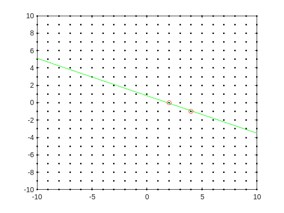
Now, some might think in terms of orthogonal distance to the line, but really, we want the vertical distance to be minimized. Again, minimize abs(delta) in the equation:
log2(3.6) + delta = p + log2(5)*q
where p and q are integer.
Can we do that using MATLAB? The skill about about mathematics often lies in formulating a word problem, and then turning the word problem into a problem of mathematics that we know how to solve. We are almost there now. I next want to formulate this into a problem that intlinprog can solve. The problem at first is intlinprog cannot handle absolute value constraints. And the trick there is to employ slack variables, a terribly useful tool to emply on this class of problem.
Rewrite delta as:
delta = Dpos - Dneg
where Dpos and Dneg are real variables, but both are constrained to be positive.
prob = optimproblem;
p = optimvar('p',lower = -50,upper = 50,type = 'integer');
q = optimvar('q',lower = -50,upper = 50,type = 'integer');
Dpos = optimvar('Dpos',lower = 0);
Dneg = optimvar('Dneg',lower = 0);
Our goal for the ILP solver will be to minimize Dpos + Dneg now. But since they must both be positive, it solves the min absolute value objective. One of them will always be zero.
r = 3.6;
prob.Constraints = log2(r) + Dpos - Dneg == p + log2(5)*q;
prob.Objective = Dpos + Dneg;
The solve is now a simple one. I'll tell it to use intlinprog, even though it would probably figure that out by itself. (Note: if I do not tell solve which solver to use, it does use intlinprog. But it also finds the correct solution when I told it to use GA offline.)
solve(prob,solver = 'intlinprog')
The solution it finds within the bounds of +/- 50 for both p and q seems pretty good. Note that Dpos and Dneg are pretty close to zero.
2^39*5^-16
and while 3.6028979... seems like nothing special, in fact, it is of the form we want.
R = sym(2)^39*sym(5)^-16
vpa(R,100)
vpa(1/R,100)
both of those numbers are exact. If I wanted to find a better approximation to 3.6, all I need do is extend the bounds on p and q. And we can use the same solution approch for any floating point number.
Check out how these charts were made with polar axes in the Graphics and App Building blog's latest article "Polar plots with patches and surface".

Nine new Image Processing courses plus one new learning path are now available as part of the Online Training Suite. These courses replace the content covered in the self-paced course Image Processing with MATLAB, which sunsets in 2026.
New courses include:
- Work with Image Data Types
- Image Registration
- Edge, Circle, and Line Detection
- Manage and Process Multiple Images
The new learning path Image Segmentation and Analysis in MATLAB earns users the digital credential Image Segmentation in MATLAB and contains the following courses:
Apparently, the back end here is running 2025b, hovering over the Run button and the Executing In popup both show R2024a.
ver matlab
Registration is now open for MathWorks annual virtual event MATLAB EXPO 2025 on November 12 – 13, 2025!
Register now and start building your customized agenda today!
Explore. Experience. Engage.
Join MATLAB EXPO to connect with MathWorks and industry experts to learn about the latest trends and advancements in engineering and science. You will discover new features and capabilities for MATLAB and Simulink that you can immediately apply to your work.

all(logical.empty)
Discuss!
I just noticed that MATLAB R2025b is available. I am a bit surprised, as I never got notification of the beta test for it.
This topic is for highlights and experiences with R2025b.
“Hello, I am Subha & I’m part of the organizing/mentoring team for NASA Space Apps Challenge Virudhunagar 2025 🚀. We’re looking for collaborators/mentors with ML and MATLAB expertise to help our student teams bring their space solutions to life. Would you be open to guiding us, even briefly? Your support could impact students tackling real NASA challenges. 🌍✨”
Since R2024b, a Levenberg–Marquardt solver (TrainingOptionsLM) was introduced. The built‑in function trainnet now accepts training options via the trainingOptions function (https://www.mathworks.com/help/deeplearning/ref/trainingoptions.html#bu59f0q-2) and supports the LM algorithm. I have been curious how to use it in deep learning, and the official documentation has not provided a concrete usage example so far. Below I give a simple example to illustrate how to use this LM algorithm to optimize a small number of learnable parameters.
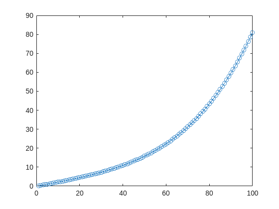
For example, consider the nonlinear function:
y_hat = @(a,t) a(1)*(t/100) + a(2)*(t/100).^2 + a(3)*(t/100).^3 + a(4)*(t/100).^4;
It represents a curve. Given 100 matching points (t → y_hat), we want to use least squares to estimate the four parameters a1–a4.
t = (1:100)';
y_hat = @(a,t)a(1)*(t/100) + a(2)*(t/100).^2 + a(3)*(t/100).^3 + a(4)*(t/100).^4;
x_true = [ 20 ; 10 ; 1 ; 50 ];
y_true = y_hat(x_true,t);
plot(t,y_true,'o-')
- Using the traditional lsqcurvefit-wrapped "Levenberg–Marquardt" algorithm:
x_guess = [ 5 ; 2 ; 0.2 ; -10 ];
options = optimoptions("lsqcurvefit",Algorithm="levenberg-marquardt",MaxFunctionEvaluations=800);
[x,resnorm,residual,exitflag] = lsqcurvefit(y_hat,x_guess,t,y_true,-50*ones(4,1),60*ones(4,1),options);
x,resnorm,exitflag
- Using the deep-learning-wrapped "Levenberg–Marquardt" algorithm:
options = trainingOptions("lm", ...
InitialDampingFactor=0.002, ...
MaxDampingFactor=1e9, ...
DampingIncreaseFactor=12, ...
DampingDecreaseFactor=0.2,...
GradientTolerance=1e-6, ...
StepTolerance=1e-6,...
Plots="training-progress");
numFeatures = 1;
layers = [featureInputLayer(numFeatures,'Name','input')
fitCurveLayer(Name='fitCurve')];
net = dlnetwork(layers);
XData = dlarray(t);
YData = dlarray(y_true);
netTrained = trainnet(XData,YData,net,"mse",options);
netTrained.Layers(2)
classdef fitCurveLayer < nnet.layer.Layer ...
& nnet.layer.Acceleratable
% Example custom SReLU layer.
properties (Learnable)
% Layer learnable parameters
a1
a2
a3
a4
end
methods
function layer = fitCurveLayer(args)
arguments
args.Name = "lm_fit";
end
% Set layer name.
layer.Name = args.Name;
% Set layer description.
layer.Description = "fit curve layer";
end
function layer = initialize(layer,~)
% layer = initialize(layer,layout) initializes the layer
% learnable parameters using the specified input layout.
if isempty(layer.a1)
layer.a1 = rand();
end
if isempty(layer.a2)
layer.a2 = rand();
end
if isempty(layer.a3)
layer.a3 = rand();
end
if isempty(layer.a4)
layer.a4 = rand();
end
end
function Y = predict(layer, X)
% Y = predict(layer, X) forwards the input data X through the
% layer and outputs the result Y.
% Y = layer.a1.*exp(-X./layer.a2) + layer.a3.*X.*exp(-X./layer.a4);
Y = layer.a1*(X/100) + layer.a2*(X/100).^2 + layer.a3*(X/100).^3 + layer.a4*(X/100).^4;
end
end
end
The network is very simple — only the fitCurveLayer defines the learnable parameters a1–a4. I observed that the output values are very close to those from lsqcurvefit.