R =
Results for
AI for Engineered Systems
47%
Cloud, Software Factories, & DevOps
0%
Electrification
13%
Autonomous Systems and Robotics
13%
Model-Based Design
7%
Wireless Communications
20%
15 votes
Yesterday I had an urgent service call for MatLab tech support. The Mathworks technician on call, Ivy Ngyuen, helped fix the problem. She was very patient and I truly appreciate her efforts, which resolved the issue. Thank you.
Hi. I'm interested to learn more about MATLAB.
excited to learn more on Mathworks
Looking forward to the Expo!
I saw an interesting problem on a reddit math forum today. The question was to find a number (x) as close as possible to r=3.6, but the requirement is that both x and 1/x be representable in a finite number of decimal places.
The problem of course is that 3.6 = 18/5. And the problem with 18/5 has an inverse 5/18, which will not have a finite representation in decimal form.
In order for a number and its inverse to both be representable in a finite number of decimal places (using base 10) we must have it be of the form 2^p*5^q, where p and q are integer, but may be either positive or negative. If that is not clear to you intuitively, suppose we have a form
2^p*5^-q
where p and q are both positive. All you need do is multiply that number by 10^q. All this does is shift the decimal point since you are just myltiplying by powers of 10. But now the result is
2^(p+q)
and that is clearly an integer, so the original number could be represented using a finite number of digits as a decimal. The same general idea would apply if p was negative, or if both of them were negative exponents.
Now, to return to the problem at hand... We can obviously adjust the number r to be 20/5 = 4, or 16/5 = 3.2. In both cases, since the fraction is now of the desired form, we are happy. But neither of them is really close to 3.6. My goal will be to find a better approximation, but hopefully, I can avoid a horrendous amount of trial and error. It would seem the trick might be to take logs, to get us closer to a solution. That is, suppose I take logs, to the base 2?
log2(3.6)
I used log2 here because that makes the problem a little simpler, since log2(2^p)=p. Therefore we want to find a pair of integers (p,q) such that
log2(3.6) + delta = p + log2(5)*q
where delta is as close to zero as possible. Thus delta is the error in our approximation to 3.6. And since we are working in logs, delta can be viewed as a proportional error term. Again, p and q may be any integers, either positive or negative. The two cases we have seen already have (p,q) = (2,0), and (4,-1).
Do you see the general idea? The line we have is of the form
log2(3.6) = p + log2(5)*q
it represents a line in the (p,q) plane, and we want to find a point on the integer lattice (p,q) where the line passes as closely as possible.
[Xl,Yl] = meshgrid([-10:10]);
plot(Xl,Yl,'k.')
hold on
fimplicit(@(p,q) -log2(3.6) + p + log2(5)*q,[-10,10,-10,10],'g-')
plot([2 4],[0,-1],'ro')
hold off
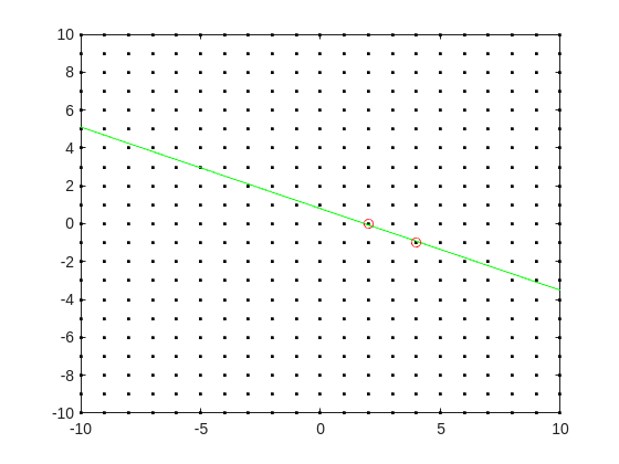
Now, some might think in terms of orthogonal distance to the line, but really, we want the vertical distance to be minimized. Again, minimize abs(delta) in the equation:
log2(3.6) + delta = p + log2(5)*q
where p and q are integer.
Can we do that using MATLAB? The skill about about mathematics often lies in formulating a word problem, and then turning the word problem into a problem of mathematics that we know how to solve. We are almost there now. I next want to formulate this into a problem that intlinprog can solve. The problem at first is intlinprog cannot handle absolute value constraints. And the trick there is to employ slack variables, a terribly useful tool to emply on this class of problem.
Rewrite delta as:
delta = Dpos - Dneg
where Dpos and Dneg are real variables, but both are constrained to be positive.
prob = optimproblem;
p = optimvar('p',lower = -50,upper = 50,type = 'integer');
q = optimvar('q',lower = -50,upper = 50,type = 'integer');
Dpos = optimvar('Dpos',lower = 0);
Dneg = optimvar('Dneg',lower = 0);
Our goal for the ILP solver will be to minimize Dpos + Dneg now. But since they must both be positive, it solves the min absolute value objective. One of them will always be zero.
r = 3.6;
prob.Constraints = log2(r) + Dpos - Dneg == p + log2(5)*q;
prob.Objective = Dpos + Dneg;
The solve is now a simple one. I'll tell it to use intlinprog, even though it would probably figure that out by itself. (Note: if I do not tell solve which solver to use, it does use intlinprog. But it also finds the correct solution when I told it to use GA offline.)
solve(prob,solver = 'intlinprog')
The solution it finds within the bounds of +/- 50 for both p and q seems pretty good. Note that Dpos and Dneg are pretty close to zero.
2^39*5^-16
and while 3.6028979... seems like nothing special, in fact, it is of the form we want.
R = sym(2)^39*sym(5)^-16
vpa(R,100)
vpa(1/R,100)
both of those numbers are exact. If I wanted to find a better approximation to 3.6, all I need do is extend the bounds on p and q. And we can use the same solution approch for any floating point number.
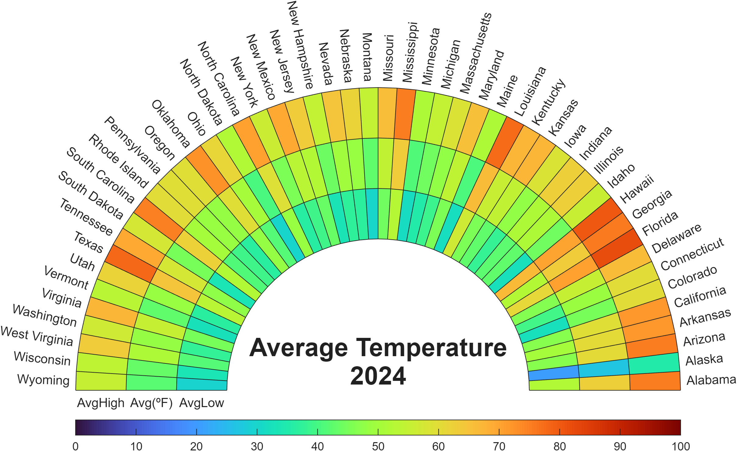
Check out how these charts were made with polar axes in the Graphics and App Building blog's latest article "Polar plots with patches and surface".

Nine new Image Processing courses plus one new learning path are now available as part of the Online Training Suite. These courses replace the content covered in the self-paced course Image Processing with MATLAB, which sunsets in 2026.
New courses include:
- Work with Image Data Types
- Image Registration
- Edge, Circle, and Line Detection
- Manage and Process Multiple Images
The new learning path Image Segmentation and Analysis in MATLAB earns users the digital credential Image Segmentation in MATLAB and contains the following courses:
Apparently, the back end here is running 2025b, hovering over the Run button and the Executing In popup both show R2024a.
ver matlab
Registration is now open for MathWorks annual virtual event MATLAB EXPO 2025 on November 12 – 13, 2025!
Register now and start building your customized agenda today!
Explore. Experience. Engage.
Join MATLAB EXPO to connect with MathWorks and industry experts to learn about the latest trends and advancements in engineering and science. You will discover new features and capabilities for MATLAB and Simulink that you can immediately apply to your work.

all(logical.empty)
Discuss!
I just noticed that MATLAB R2025b is available. I am a bit surprised, as I never got notification of the beta test for it.
This topic is for highlights and experiences with R2025b.
“Hello, I am Subha & I’m part of the organizing/mentoring team for NASA Space Apps Challenge Virudhunagar 2025 🚀. We’re looking for collaborators/mentors with ML and MATLAB expertise to help our student teams bring their space solutions to life. Would you be open to guiding us, even briefly? Your support could impact students tackling real NASA challenges. 🌍✨”
Since R2024b, a Levenberg–Marquardt solver (TrainingOptionsLM) was introduced. The built‑in function trainnet now accepts training options via the trainingOptions function (https://www.mathworks.com/help/deeplearning/ref/trainingoptions.html#bu59f0q-2) and supports the LM algorithm. I have been curious how to use it in deep learning, and the official documentation has not provided a concrete usage example so far. Below I give a simple example to illustrate how to use this LM algorithm to optimize a small number of learnable parameters.
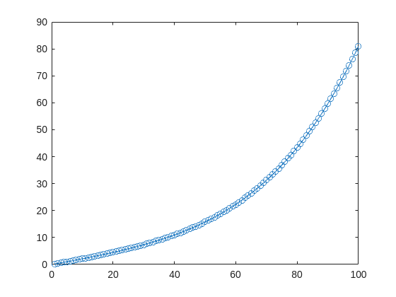
For example, consider the nonlinear function:
y_hat = @(a,t) a(1)*(t/100) + a(2)*(t/100).^2 + a(3)*(t/100).^3 + a(4)*(t/100).^4;
It represents a curve. Given 100 matching points (t → y_hat), we want to use least squares to estimate the four parameters a1–a4.
t = (1:100)';
y_hat = @(a,t)a(1)*(t/100) + a(2)*(t/100).^2 + a(3)*(t/100).^3 + a(4)*(t/100).^4;
x_true = [ 20 ; 10 ; 1 ; 50 ];
y_true = y_hat(x_true,t);
plot(t,y_true,'o-')
- Using the traditional lsqcurvefit-wrapped "Levenberg–Marquardt" algorithm:
x_guess = [ 5 ; 2 ; 0.2 ; -10 ];
options = optimoptions("lsqcurvefit",Algorithm="levenberg-marquardt",MaxFunctionEvaluations=800);
[x,resnorm,residual,exitflag] = lsqcurvefit(y_hat,x_guess,t,y_true,-50*ones(4,1),60*ones(4,1),options);
x,resnorm,exitflag
- Using the deep-learning-wrapped "Levenberg–Marquardt" algorithm:
options = trainingOptions("lm", ...
InitialDampingFactor=0.002, ...
MaxDampingFactor=1e9, ...
DampingIncreaseFactor=12, ...
DampingDecreaseFactor=0.2,...
GradientTolerance=1e-6, ...
StepTolerance=1e-6,...
Plots="training-progress");
numFeatures = 1;
layers = [featureInputLayer(numFeatures,'Name','input')
fitCurveLayer(Name='fitCurve')];
net = dlnetwork(layers);
XData = dlarray(t);
YData = dlarray(y_true);
netTrained = trainnet(XData,YData,net,"mse",options);
netTrained.Layers(2)
classdef fitCurveLayer < nnet.layer.Layer ...
& nnet.layer.Acceleratable
% Example custom SReLU layer.
properties (Learnable)
% Layer learnable parameters
a1
a2
a3
a4
end
methods
function layer = fitCurveLayer(args)
arguments
args.Name = "lm_fit";
end
% Set layer name.
layer.Name = args.Name;
% Set layer description.
layer.Description = "fit curve layer";
end
function layer = initialize(layer,~)
% layer = initialize(layer,layout) initializes the layer
% learnable parameters using the specified input layout.
if isempty(layer.a1)
layer.a1 = rand();
end
if isempty(layer.a2)
layer.a2 = rand();
end
if isempty(layer.a3)
layer.a3 = rand();
end
if isempty(layer.a4)
layer.a4 = rand();
end
end
function Y = predict(layer, X)
% Y = predict(layer, X) forwards the input data X through the
% layer and outputs the result Y.
% Y = layer.a1.*exp(-X./layer.a2) + layer.a3.*X.*exp(-X./layer.a4);
Y = layer.a1*(X/100) + layer.a2*(X/100).^2 + layer.a3*(X/100).^3 + layer.a4*(X/100).^4;
end
end
end
The network is very simple — only the fitCurveLayer defines the learnable parameters a1–a4. I observed that the output values are very close to those from lsqcurvefit.
I’d like to take a moment to highlight the great contributions of one of our community members, @Paul, who is fast approaching an impressive 5,000 reputation points!
Paul has built his reputation the best way possible - by generously sharing his knowledge and helping others. Over the last few years, he’s provided thoughtful and practical answers to hundreds of questions, making life a little easier for learners and experts alike.
Reputation points are more than just numbers here - they represent the trust and appreciation of the community. Paul’s upcoming milestone is a testament to his consistency, expertise, and willingness to support others.
Please join me in recognizing Paul's contributions and impact on the MATLAB Central community.
Function Syntax Design Conundrum
As a MATLAB enthusiast, I particularly enjoy Steve Eddins' blog and the cool things he explores. MATLAB's new argument blocks are great, but there's one frustrating limitation that Steve outlined beautifully in his blog post "Function Syntax Design Conundrum": cases where an argument should accept both enumerated values AND other data types.
Steve points out this could be done using the input parser, but I prefer having tab completions and I'm not a fan of maintaining function signature JSON files for all my functions.
Personal Context on Enumerations
To be clear: I honestly don't like enumerations in any way, shape, or form. One reason is how awkward they are. I've long suspected they're simply predefined constructor calls with a set argument, and I think that's all but confirmed here. This explains why I've had to fight the enumeration system when trying to take arguments of many types and normalize them to enumerated members, or have numeric values displayed as enumerated members without being recast to the superclass every operation.
The Discovery
While playing around extensively with metadata for another project, I realized (and I'm entirely unsure why it took so long) that the properties of a metaclass object are just, in many cases, the attributes of the classdef. In this realization, I found a solution to Steve's and my problem.
To be clear: I'm not in love with this solution. I would much prefer a better approach for allowing variable sets of membership validation for arguments. But as it stands, we don't have that, so here's an interesting, if incredibly hacky, solution.
If you call struct() on a metaclass object to view its hidden properties, you'll notice that in addition to the public "Enumeration" property, there's a hidden "Enumerable" property. They're both logicals, which implies they're likely functionally distinct. I was curious about that distinction and hoped to find some functionality by intentionally manipulating these values - and I did, solving the exact problem Steve mentions.
The Problem Statement
We have a function with an argument that should allow "dual" input types: enumerated values (Steve's example uses days of the week, mine uses the "all" option available in various dimension-operating functions) AND integers. We want tab completion for the enumerated values while still accepting the numeric inputs.
A Solution for Tab-Completion Supported Arguments
Rather than spoil Steve's blog post, let me use my own example: implementing a none() function. The definition is simple enough tf = ~any(A, dim); but when we wrap this in another function, we lose the tab-completion that any() provides for the dim argument (which gives you "all"). There's no great way to implement this as a function author currently - at least, that's well documented.
So here's my solution:
%% Example Function Implementation
% This is a simple implementation of the DimensionArgument class for implementing dual type inputs that allow enumerated tab-completion.
function tf = none(A, dim)
arguments(Input)
A logical;
dim DimensionArgument = DimensionArgument(A, true);
end
% Simple example (notice the use of uplus to unwrap the hidden property)
tf = ~any(A, +dim);
end
I like this approach because the additional work required to implement it, once the enumeration class is initialized, is minimal. Here are examples of function calls, note that the behavior parallels that of the MATLAB native-style tab-completion:
%% Test Data
% Simple logical array for testing
A = randi([0, 1], [3, 5], "logical");
%% Example function calls
tf = none(A, "all"); % This is the tab-completion it's 1:1 with MATLABs behavior
tf = none(A, [1, 2]); % We can still use valid arguments (validated in the constructor)
tf = none(A); % Showcase of the constructors use as a default argument generator
How It Works
What makes this work is the previously mentioned Enumeration attribute. By setting Enumeration = false while still declaring an enumeration block in the classdef file, we get the suggested members as auto-complete suggestions. As I hinted at, the value of enumerations (if you don't subclass a builtin and define values with the someMember (1) syntax) are simply arguments to constructor calls.
We also get full control over the storage and handling of the class, which means we lose the implicit storage that enumerations normally provide and are responsible for doing so ourselves - but I much prefer this. We can implement internal validation logic to ensure values that aren't in the enumerated set still comply with our constraints, and store the input (whether the enumerated member or alternative type) in an internal property.
As seen in the example class below, this maintains a convenient interface for both the function caller and author the only particuarly verbose portion is the conversion methods... Which if your willing to double down on the uplus unwrapping context can be avoided. What I have personally done is overload the uplus function to return the input (or perform the identity property) this allowss for the uplus to be used universally to unwrap inputs and for those that cant, and dont have a uplus definition, the value itself is just returned:
classdef(Enumeration = false) DimensionArgument % < matlab.mixin.internal.MatrixDisplay
%DimensionArgument Enumeration class to provide auto-complete on functions needing the dimension type seen in all()
% Enumerations are just macros to make constructor calls with a known set of arguments. Declaring the 'all'
% enumeration member means this class can be set as the type for an input and the auto-completion for the given
% argument will show the enumeration members, allowing tab-completion. Declaring the Enumeration attribute of
% the class as false gives us control over the constructor and internal implementation. As such we can use it
% to validate the numeric inputs, in the event the 'all' option was not used, and return an object that will
% then work in place of valid dimension argument options.
%% Enumeration members
% These are the auto-complete options you'd like to make available for the function signature for a given
% argument.
enumeration(Description="Enumerated value for the dimension argument.")
all
end
%% Properties
% The internal property allows the constructor's input to be stored; this ensures that the value is store and
% that the output of the constructor has the class type so that the validation passes.
% (Constructors must return the an object of the class they're a constructor for)
properties(Hidden, Description="Storage of the constructor input for later use.")
Data = [];
end
%% Constructor method
% By the magic of declaring (Enumeration = false) in our class def arguments we get full control over the
% constructor implementation.
%
% The second argument in this specific instance is to enable the argument's default value to be set in the
% arguments block itself as opposed to doing so in the function body... I like this better but if you didn't
% you could just as easily keep the constructor simple.
methods
function obj = DimensionArgument(A, Adim)
%DimensionArgument Initialize the dimension argument.
arguments
% This will be the enumeration member name from auto-completed entries, or the raw user input if not
% used.
A = [];
% A flag that indicates to create the value using different logic, in this case the first non-singleton
% dimension, because this matches the behavior of functions like, all(), sum() prod(), etc.
Adim (1, 1) logical = false;
end
if(Adim)
% Allows default initialization from an input to match the aforemention function's behavior
obj.Data = firstNonscalarDim(A);
else
% As a convenience for this style of implementation we can validate the input to ensure that since we're
% suppose to be an enumeration, the input is valid
DimensionArgument.mustBeValidMember(A);
% Store the input in a hidden property since declaring ~Enumeration means we are responsible for storing
% it.
obj.Data = A;
end
end
end
%% Conversion methods
% Applies conversion to the data property so that implicit casting of functions works. Unfortunately most of
% the MathWorks defined functions use a different system than that employed by the arguments block, which
% defers to the class defined converter methods... Which is why uplus (+obj) has been defined to unwrap the
% data for ease of use.
methods
function obj = uplus(obj)
obj = obj.Data;
end
function str = char(obj)
str = char(obj.Data);
end
function str = cellstr(obj)
str = cellstr(obj.Data);
end
function str = string(obj)
str = string(obj.Data);
end
function A = double(obj)
A = double(obj.Data);
end
function A = int8(obj)
A = int8(obj.Data);
end
function A = int16(obj)
A = int16(obj.Data);
end
function A = int32(obj)
A = int32(obj.Data);
end
function A = int64(obj)
A = int64(obj.Data);
end
end
%% Validation methods
% These utility methods are for input validation
methods(Static, Access = private)
function tf = isValidMember(obj)
%isValidMember Checks that the input is a valid dimension argument.
tf = (istext(obj) && all(obj == "all", "all")) || (isnumeric(obj) && all(isint(obj) & obj > 0, "all"));
end
function mustBeValidMember(obj)
%mustBeValidMember Validates that the input is a valid dimension argument for the dim/dimVec arguments.
if(~DimensionArgument.isValidMember(obj))
exception("JB:DimensionArgument:InvalidInput", "Input must be an integer value or the term 'all'.")
end
end
end
%% Convenient data display passthrough
methods
function disp(obj, name)
arguments
obj DimensionArgument
name string {mustBeScalarOrEmpty} = [];
end
% Dispatch internal data's display implementation
display(obj.Data, char(name));
end
end
end
In the event you'd actually play with theres here are the function definitions for some of the utility functions I used in them, including my exception would be a pain so i wont, these cases wont use it any...
% Far from my definition isint() but is consistent with mustBeInteger() for real numbers but will suffice for the example
function tf = isint(A)
arguments
A {mustBeNumeric(A)};
end
tf = floor(A) == A
end
% Sort of the same but its fine
function dim = firstNonscalarDim(A)
arguments
A
end
dim = [find(size(A) > 1, 1), 0];
dim(1) = dim(1);
end
Hello MATLAB Central, this is my first article.
My name is Yann. And I love MATLAB.
I also love HTTP (i know, weird fetish)
So i started a conversation with ChatGPT about it:
gitclone('https://github.com/yanndebray/HTTP-with-MATLAB');
cd('HTTP-with-MATLAB')
http_with_MATLAB
I'm not sure that this platform is intended to clone repos from github, but i figured I'd paste this shortcut in case you want to try out my live script http_with_MATLAB.m
A lot of what i program lately relies on external web services (either for fetching data, or calling LLMs).
So I wrote a small tutorial of the 7 or so things I feel like I need to remember when making HTTP requests in MATLAB.
Let me know what you think
a = [ 1 2 3 ]
a =
1 2 3
b = [ 3; 5; 8]
b =
3
5
8
x = a + b
x =
4 5 6
6 7 8
9 10 11
I can not understand why Plot Browser was taken away in latest Matlab... I use Plot Browser all of the time! Having to find and click the particular line I want in a plot with a lot of lines is way less convenient than just selecting it in the Plot Browser. Also, being able to quickly hide/show multiple lines at once with the plot browser was so helpful in a lot of cases. Please bring Plot Browser back!!!! Please reply with support for this if you feel the same as I do!
In the latest Graphics and App Building blog article, documentation writer Jasmine Poppick modernized a figure-based bridge analysis app by replacing uicontrol with new UI components and uifigure, resulting in cleaner code, better layouts, and expanded functionality in R2025a.
https://blogs.mathworks.com/graphics-and-apps/2025/08/19/__from-uicontrol-to-ui-components
This article covers the following topics:
Why and when to move from uicontrol and figure to modern UI components and uifigure.
How to replace uicontrol objects with equivalent UI component functions (uicheckbox, uidropdown, uispinner, etc.).
How to update callback code to match new component properties and behaviors.
How to adopt new UI component types (like spinners) to simplify validation and improve usability.
How to configure existing components with modern options (sortable tables, auto-fitting columns, editable data).
How to apply visual styling with uistyle and addStyle to make apps more user-friendly.
How to use uigridlayout to create flexible, adaptive layouts instead of manually managing positions.
The benefits of switching from figure to uifigure for app-building workflows.
A full before-and-after example of modernizing an existing app with incremental, practical updates.