Results for
When you compare MATLAB Plot Gallery with matplotlib gallery, you can see that matplotlib gallery contains a lot of nice graphs which are easy to create in MATLAB but not listed in MATLAB Plot Gallery.
For example, "Data Distribution Plots" section in the MATLAB Plot Gallery includes example for pie function instead of examples for piechart and donutchart functions, etc.
Did you know that function double with string vector input significantly outperforms str2double with the same input:
x = rand(1,50000);
t = string(x);
tic; str2double(t); toc
tic; I1 = str2double(t); toc
tic; I2 = double(t); toc
isequal(I1,I2)
Recently I needed to parse numbers from text. I automatically tried to use str2double. However, profiling revealed that str2double was the main bottleneck in my code. Than I realized that there is a new note (since R2024a) in the documentation of str2double:
"Calling string and then double is recommended over str2double because it provides greater flexibility and allows vectorization. For additional information, see Alternative Functionality."
mlapp being a binary is a pain point for source control. It means that you either have to:
- have hooks in your source control system to zip/unzip a mlapp. However, The Mathworks have informed users not to rely on this as the mlapp format may change.
- do all your source control in MATLAB. This is non standard behaviour. Source code and source control should be independent of each other. Web front-ends to source control systems, 3rd party source control apps, CI/CD systems and much more are extremely limited in what they can do with mlapps.
I wish an mlapp could just be a directory full of the required text/other files.
Requested to post this here from reddit.
There is no call to rescan audio devices in audioPlayerRecorder, even though PortAudio has such a call. I have a measurement environment that takes a long time to initialise. If I forget to plug in my audio device, I have to do it all over again...
Share your ideas, suggestions, and wishlists for improving MathWorks products. What would make the software absolutely perfect for you? Discuss your idea(s) with other community users.
Guidelines & Tips
We encourage all ideas, big or small! To help everyone understand and discuss your suggestion, please include as much detail as possible in your post:
- Product or Feature: Clearly state which product (e.g., MATLAB, Simulink, a toolbox, etc.) or specific feature your idea relates to.
- The Problem or Opportunity: Briefly describe what challenge you’re facing or what opportunity you see for improvement.
- Your Idea: Explain your suggestion in detail. What would you like to see added, changed, or improved? How would it help you and other users?
- Examples or Use Cases (optional): If possible, include an example, scenario, or workflow to illustrate your idea.
- Related Posts (optional): If you’ve seen similar ideas or discussions, feel free to link to them for context.
Ready to share your idea?
Click here and then "Start a Discussion”, and let the community know how MATLAB could be even better for you!
Thank you for your contributions and for helping make MATLAB Central a vibrant place for sharing and improving ideas.
Hey cody fellows :-) !
I recently created two problem groups, but as you can see I struggle to set their cover images :
What is weird given :
- I already did it successfully twice in the past for my previous groups ;
- If you take one problem specifically, Problem 60984. Mesh the icosahedron for instance, you can normally see the icon of the cover image in the top right hand corner, can't you ?
- I always manage to set cover images to my contributions (mostly in the filexchange).
I already tried several image formats, included .png 4/3 ratio, but still the cover images don't set.
Could you please help me to correctly set my cover images ?
Thank you.
Nicolas
Resharing a fun short video explaining what MATLAB is. :)
t = turtle(); % Start a turtle
t.forward(100); % Move forward by 100
t.backward(100); % Move backward by 100
t.left(90); % Turn left by 90 degrees
t.right(90); % Tur right by 90 degrees
t.goto(100, 100); % Move to (100, 100)
t.turnto(90); % Turn to 90 degrees, i.e. north
t.speed(1000); % Set turtle speed as 1000 (default: 500)
t.pen_up(); % Pen up. Turtle leaves no trace.
t.pen_down(); % Pen down. Turtle leaves a trace again.
t.color('b'); % Change line color to 'b'
t.begin_fill(FaceColor, EdgeColor, FaceAlpha); % Start filling
t.end_fill(); % End filling
t.change_icon('person.png'); % Change the icon to 'person.png'
t.clear(); % Clear the Axes
classdef turtle < handle
properties (GetAccess = public, SetAccess = private)
x = 0
y = 0
q = 0
end
properties (SetAccess = public)
speed (1, 1) double = 500
end
properties (GetAccess = private)
speed_reg = 100
n_steps = 20
ax
l
ht
im
is_pen_up = false
is_filling = false
fill_color
fill_alpha
end
methods
function obj = turtle()
figure(Name='MATurtle', NumberTitle='off')
obj.ax = axes(box="on");
hold on,
obj.ht = hgtransform();
icon = flipud(imread('turtle.png'));
obj.im = imagesc(obj.ht, icon, ...
XData=[-30, 30], YData=[-30, 30], ...
AlphaData=(255 - double(rgb2gray(icon)))/255);
obj.l = plot(obj.x, obj.y, 'k');
obj.ax.XLim = [-500, 500];
obj.ax.YLim = [-500, 500];
obj.ax.DataAspectRatio = [1, 1, 1];
obj.ax.Toolbar.Visible = 'off';
disableDefaultInteractivity(obj.ax);
end
function home(obj)
obj.x = 0;
obj.y = 0;
obj.ht.Matrix = eye(4);
end
function forward(obj, dist)
obj.step(dist);
end
function backward(obj, dist)
obj.step(-dist)
end
function step(obj, delta)
if numel(delta) == 1
delta = delta*[cosd(obj.q), sind(obj.q)];
end
if obj.is_filling
obj.fill(delta);
else
obj.move(delta);
end
end
function goto(obj, x, y)
dx = x - obj.x;
dy = y - obj.y;
obj.turnto(rad2deg(atan2(dy, dx)));
obj.step([dx, dy]);
end
function left(obj, q)
obj.turn(q);
end
function right(obj, q)
obj.turn(-q);
end
function turnto(obj, q)
obj.turn(obj.wrap_angle(q - obj.q, -180));
end
function pen_up(obj)
if obj.is_filling
warning('not available while filling')
return
end
obj.is_pen_up = true;
end
function pen_down(obj, go)
if obj.is_pen_up
if nargin == 1
obj.l(end+1) = plot(obj.x, obj.y, Color=obj.l(end).Color);
else
obj.l(end+1) = go;
end
uistack(obj.ht, 'top')
end
obj.is_pen_up = false;
end
function color(obj, line_color)
if obj.is_filling
warning('not available while filling')
return
end
obj.pen_up();
obj.pen_down(plot(obj.x, obj.y, Color=line_color));
end
function begin_fill(obj, FaceColor, EdgeColor, FaceAlpha)
arguments
obj
FaceColor = [.6, .9, .6];
EdgeColor = [0 0.4470 0.7410];
FaceAlpha = 1;
end
if obj.is_filling
warning('already filling')
return
end
obj.fill_color = FaceColor;
obj.fill_alpha = FaceAlpha;
obj.pen_up();
obj.pen_down(patch(obj.x, obj.y, [1, 1, 1], ...
EdgeColor=EdgeColor, FaceAlpha=0));
obj.is_filling = true;
end
function end_fill(obj)
if ~obj.is_filling
warning('not filling now')
return
end
obj.l(end).FaceColor = obj.fill_color;
obj.l(end).FaceAlpha = obj.fill_alpha;
obj.is_filling = false;
end
function change_icon(obj, filename)
icon = flipud(imread(filename));
obj.im.CData = icon;
obj.im.AlphaData = (255 - double(rgb2gray(icon)))/255;
end
function clear(obj)
obj.x = 0;
obj.y = 0;
delete(obj.ax.Children(2:end));
obj.l = plot(0, 0, 'k');
obj.ht.Matrix = eye(4);
end
end
methods (Access = private)
function animated_step(obj, delta, q, initFcn, updateFcn)
arguments
obj
delta
q
initFcn = @() []
updateFcn = @(~, ~) []
end
dx = delta(1)/obj.n_steps;
dy = delta(2)/obj.n_steps;
dq = q/obj.n_steps;
pause_duration = norm(delta)/obj.speed/obj.speed_reg;
initFcn();
for i = 1:obj.n_steps
updateFcn(dx, dy);
obj.ht.Matrix = makehgtform(...
translate=[obj.x + dx*i, obj.y + dy*i, 0], ...
zrotate=deg2rad(obj.q + dq*i));
pause(pause_duration)
drawnow limitrate
end
obj.x = obj.x + delta(1);
obj.y = obj.y + delta(2);
end
function obj = turn(obj, q)
obj.animated_step([0, 0], q);
obj.q = obj.wrap_angle(obj.q + q, 0);
end
function move(obj, delta)
initFcn = @() [];
updateFcn = @(dx, dy) [];
if ~obj.is_pen_up
initFcn = @() initializeLine();
updateFcn = @(dx, dy) obj.update_end_point(obj.l(end), dx, dy);
end
function initializeLine()
obj.l(end).XData(end+1) = obj.l(end).XData(end);
obj.l(end).YData(end+1) = obj.l(end).YData(end);
end
obj.animated_step(delta, 0, initFcn, updateFcn);
end
function obj = fill(obj, delta)
initFcn = @() initializePatch();
updateFcn = @(dx, dy) obj.update_end_point(obj.l(end), dx, dy);
function initializePatch()
obj.l(end).Vertices(end+1, :) = obj.l(end).Vertices(end, :);
obj.l(end).Faces = 1:size(obj.l(end).Vertices, 1);
end
obj.animated_step(delta, 0, initFcn, updateFcn);
end
end
methods (Static, Access = private)
function update_end_point(l, dx, dy)
l.XData(end) = l.XData(end) + dx;
l.YData(end) = l.YData(end) + dy;
end
function q = wrap_angle(q, min_angle)
q = mod(q - min_angle, 360) + min_angle;
end
end
end
Nice to have - function output argument provide code assist when said function is called
This is a feature which doesn't apear to currently exist, but I think alot of matlab users would like, particularly ones who write alot of custom classes.
Imagine i have a custom class with some properties:
classdef CustomClass < handle
properties
name (1,1) string = "default name"
varOne (1,1) double = 0
end
methods
function obj = CustomClass(name,varOne)
obj.name = name;
obj.VarOne = varOne;
end
end
end
Then imagine I have a function which returns one of these custom class objects:
function [obj] = Calculation(Var1,Var2,name)
arguments (Input)
Var1 (1,1) double
Var2 (1,1) double
end
arguments (Output)
obj (1,1) CustomClass
end
results = Var1 + Var2;
obj = CustomClass(name,result);
end
With this class and this function which returns one of these class objects, I would like the fact that I provided "(1,1) CustomClass" in the output arguemnts block of function "Calculation(Var1,Var2,name)" to trigger code assist automaticaly show me, when writing code that the retuned value from this funciton has properties "name" and "varOne" in the object.
For istance, if I write the following code with this function and the class in the Matlab search path
testObj = Calculation(1,1,"test");
testObj.varOne = 10; %the property "varOne" doesn't apear in code assist when writing this line of code
I would like that the fact function "Calcuation(Var1,Var2,name) has the output arguments block enforcing that this function must return an object of "CustomClass" to make code assist recognise that "testObj" is a "CustomClass" object, just as if testObj was an input argument to another function which had an input argument requiring that "testObj" was a "CustomClass" object.
Maybe this is a feature that may be added to matlab in future releases? (please and thank you LOL)
I would like to zoom directly on the selected region when using  on my image created with image or imagesc. First of all, I would recommend using image or imagesc and not imshow for this case, see comparison here: Differences between imshow() and image()? However when zooming Stretch-to-Fill behavior happens and I don't want that. Try range zoom to image generated by this code:
fig = uifigure;
ax = uiaxes(fig);
im = imread("peppers.png");
h = imagesc(im,"Parent",ax);
axis(ax,'tight', 'off')
I can fix that with manualy setting data aspect ratio:
daspect(ax,[1 1 1])
However, I need this code to run automatically after zooming. So I create zoom object and ActionPostCallback which is called everytime after I zoom, see zoom - ActionPostCallback.
z = zoom(ax);
z.ActionPostCallback = @(fig,ax) daspect(ax.Axes,[1 1 1]);
If you need, you can also create ActionPreCallback which is called everytime before I zoom, see zoom - ActionPreCallback.
z.ActionPreCallback = @(fig,ax) daspect(ax.Axes,'auto');
Code written and run in R2025a.
I am thrilled python interoperability now seems to work for me with my APPLE M1 MacBookPro and MATLAB V2025a. The available instructions are still, shall we say, cryptic. Here is a summary of my interaction with GPT 4o to get this to work.
===========================================================
MATLAB R2025a + Python (Astropy) Integration on Apple Silicon (M1/M2/M3 Macs)
===========================================================
Author: D. Carlsmith, documented with ChatGPT
Last updated: July 2025
This guide provides full instructions, gotchas, and workarounds to run Python 3.10 with MATLAB R2025a (Apple Silicon/macOS) using native ARM64 Python and calling modules like Astropy, Numpy, etc. from within MATLAB.
===========================================================
Overview
===========================================================
- MATLAB R2025a on Apple Silicon (M1/M2/M3) runs as "maca64" (native ARM64).
- To call Python from MATLAB, the Python interpreter must match that architecture (ARM64).
- Using Intel Python (x86_64) with native MATLAB WILL NOT WORK.
- The cleanest solution: use Miniforge3 (Conda-forge's lightweight ARM64 distribution).
===========================================================
1. Install Miniforge3 (ARM64-native Conda)
===========================================================
In Terminal, run:
curl -LO https://github.com/conda-forge/miniforge/releases/latest/download/Miniforge3-MacOSX-arm64.sh
bash Miniforge3-MacOSX-arm64.sh
Follow prompts:
- Press ENTER to scroll through license.
- Type "yes" when asked to accept the license.
- Press ENTER to accept the default install location: ~/miniforge3
- When asked:
Do you wish to update your shell profile to automatically initialize conda? [yes|no]
Type: yes
===========================================================
2. Restart Terminal and Create a Python Environment for MATLAB
===========================================================
Run the following:
conda create -n matlab python=3.10 astropy numpy -y
conda activate matlab
Verify the Python path:
which python
Expected output:
/Users/YOURNAME/miniforge3/envs/matlab/bin/python
===========================================================
3. Verify Python + Astropy From Terminal
===========================================================
Run:
python -c "import astropy; print(astropy.__version__)"
Expected output:
6.x.x (or similar)
===========================================================
4. Configure MATLAB to Use This Python
===========================================================
In MATLAB R2025a (Apple Silicon):
clear classes
pyenv('Version', '/Users/YOURNAME/miniforge3/envs/matlab/bin/python')
py.sys.version
You should see the Python version printed (e.g. 3.10.18). No error means it's working.
===========================================================
5. Gotchas and Their Solutions
===========================================================
❌ Error: Python API functions are not available
→ Cause: Wrong architecture or broken .dylib
→ Fix: Use Miniforge ARM64 Python. DO NOT use Intel Anaconda.
❌ Error: Invalid text character (↑ points at __version__)
→ Cause: MATLAB can’t parse double underscores typed or pasted
→ Fix: Use: py.getattr(module, '__version__')
❌ Error: Unrecognized method 'separation' or 'sec'
→ Cause: MATLAB can't reflect dynamic Python methods
→ Fix: Use: py.getattr(obj, 'method')(args)
===========================================================
6. Run Full Verification in MATLAB
===========================================================
Paste this into MATLAB:
% Set environment
clear classes
pyenv('Version', '/Users/YOURNAME/miniforge3/envs/matlab/bin/python');
% Import modules
coords = py.importlib.import_module('astropy.coordinates');
time_mod = py.importlib.import_module('astropy.time');
table_mod = py.importlib.import_module('astropy.table');
% Astropy version
ver = char(py.getattr(py.importlib.import_module('astropy'), '__version__'));
disp(['Astropy version: ', ver]);
% SkyCoord angular separation
c1 = coords.SkyCoord('10h21m00s', '+41d12m00s', pyargs('frame', 'icrs'));
c2 = coords.SkyCoord('10h22m00s', '+41d15m00s', pyargs('frame', 'icrs'));
sep_fn = py.getattr(c1, 'separation');
sep = sep_fn(c2);
arcsec = double(sep.to('arcsec').value);
fprintf('Angular separation = %.3f arcsec\n', arcsec);
% Time difference in seconds
Time = time_mod.Time;
t1 = Time('2025-01-01T00:00:00', pyargs('format','isot','scale','utc'));
t2 = Time('2025-01-02T00:00:00', pyargs('format','isot','scale','utc'));
dt = py.getattr(t2, '__sub__')(t1);
seconds = double(py.getattr(dt, 'sec'));
fprintf('Time difference = %.0f seconds\n', seconds);
% Astropy table display
tbl = table_mod.Table(pyargs('names', {'a','b'}, 'dtype', {'int','float'}));
tbl.add_row({1, 2.5});
tbl.add_row({2, 3.7});
disp(tbl);
===========================================================
7. Optional: Automatically Configure Python in startup.m
===========================================================
To avoid calling pyenv() every time, edit your MATLAB startup:
edit startup.m
Add:
try
pyenv('Version', '/Users/YOURNAME/miniforge3/envs/matlab/bin/python');
catch
warning("Python already loaded.");
end
===========================================================
8. Final Notes
===========================================================
- This setup avoids all architecture mismatches.
- It uses a clean, minimal ARM64 Python that integrates seamlessly with MATLAB.
- Do not mix Anaconda (Intel) with Apple Silicon MATLAB.
- Use py.getattr for any Python attribute containing underscores or that MATLAB can't resolve.
You can now run NumPy, Astropy, Pandas, Astroquery, Matplotlib, and more directly from MATLAB.
===========================================================
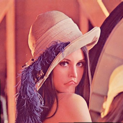
Hey MATLAB enthusiasts!
I just stumbled upon this hilariously effective GitHub repo for image deformation using Moving Least Squares (MLS)—and it’s pure gold for anyone who loves playing with pixels! 🎨✨
- Real-Time Magic ✨
- Precomputes weights and deformation data upfront, making it blazing fast for interactive edits. Drag control points and watch the image warp like rubber! (2)
- Supports affine, similarity, and rigid deformations—because why settle for one flavor of chaos?
- Single-File Simplicity 🧩
- All packed into one clean MATLAB class (mlsImageWarp.m).
- Endless Fun Use Cases 🤹
- Turn your pet’s photo into a Picasso painting.
- "Fix" your friend’s smile... aggressively.
- Animate static images with silly deformations (1).
Try the Demo!
You are not a jedi yet !
20%
We not grant u the rank of master !
0%
Ready are u? What knows u of ready?
0%
May the Force be with you !
80%
5 votes
Untapped Potential for Output-arguments Block
MATLAB has a very powerful feature in its arguments blocks. For example, the following code for a function (or method):
- clearly outlines all the possible inputs
- provides default values for each input
- will produce auto-complete suggestions while typing in the Editor (and Command Window in newer versions)
- checks each input against validation functions to enforce size, shape (e.g., column vs. row vector), type, and other options (e.g., being a member of a set)
function [out] = sample_fcn(in)
arguments(Input)
in.x (:, 1) = []
in.model_type (1, 1) string {mustBeMember(in.model_type, ...
["2-factor", "3-factor", "4-factor"])} = "2-factor"
in.number_of_terms (1, 1) {mustBeMember(in.number_of_terms, 1:5)} = 1
in.normalize_fit (1, 1) logical = false
end
% function logic ...
end
If you do not already use the arguments block for function (or method) inputs, I strongly suggest that you try it out.
The point of this post, though, is to suggest improvements for the output-arguments block, as it is not nearly as powerful as its input-arguments counterpart. I have included two function examples: the first can work in MATLAB while the second does not, as it includes suggestions for improvements. Commentary specific to each function is provided completely before the code. While this does necessitate navigating back and forth between functions and text, this provides for an easy comparison between the two functions which is my main goal.
Current Implementation
The input-arguments block for sample_fcn begins the function and has already been discussed. A simple output-arguments block is also included. I like to use a single output so that additional fields may be added at a later point. Using this approach simplifies future development, as the function signature, wherever it may be used, does not need to be changed. I can simply add another output field within the function and refer to that additional field wherever the function output is used.
Before beginning any logic, sample_fcn first assigns default values to four fields of out. This is a simple and concise way to ensure that the function will not error when returning early.
The function then performs two checks. The first is for an empty input (x) vector. If that is the case, nothing needs to be done, as the function simply returns early with the default output values that happen to apply to the inability to fit any data.
The second check is for edge cases for which input combinations do not work. In this case, the status is updated, but default values for all other output fields (which are already assigned) still apply, so no additional code is needed.
Then, the function performs the fit based on the specified model_type. Note that an otherwise case is not needed here, since the argument validation for model_type would not allow any other value.
At this point, the total_error is calculated and a check is then made to determine if it is valid. If not, the function again returns early with another specific status value.
Finally, the R^2 value is calculated and a fourth check is performed. If this one fails, another status value is assigned with an early return.
If the function has passed all the checks, then a set of assertions ensure that each of the output fields are valid. In this case, there are eight specific checks, two for each field.
If all of the assertions also pass, then the final (successful) status is assigned and the function returns normally.
function [out] = sample_fcn(in)
arguments(Input)
in.x (:, 1) = []
in.model_type (1, 1) string {mustBeMember(in.model_type, ...
["2-factor", "3-factor", "4-factor"])} = "2-factor"
in.number_of_terms (1, 1) {mustBeMember(in.number_of_terms, 1:5)} = 1
in.normalize_fit (1, 1) logical = false
end
arguments(Output)
out struct
end
%%
out.fit = [];
out.total_error = [];
out.R_squared = NaN;
out.status = "Fit not possible for supplied inputs.";
%%
if isempty(in.x)
return
end
%%
if ((in.model_type == "2-factor") && (in.number_of_terms == 5)) || ... % other possible logic
out.status = "Specified combination of model_type and number_of_terms is not supported.";
return
end
%%
switch in.model_type
case "2-factor"
out.fit = % code for 2-factor fit
case "3-factor"
out.fit = % code for 3-factor fit
case "4-factor"
out.fit = % code for 4-factor fit
end
%%
out.total_error = % calculation of error
if ~isfinite(out.total_error)
out.status = "The total_error could not be calculated.";
return
end
%%
out.R_squared = % calculation of R^2
if out.R_squared > 1
out.status = "The R^2 value is out of bounds.";
return
end
%%
assert(iscolumn(out.fit), "The fit vector is not a column vector.");
assert(size(out.fit) == size(in.x), "The fit vector is not the same size as the input x vector.");
assert(isscalar(out.total_error), "The total_error is not a scalar.");
assert(isfinite(out.total_error), "The total_error is not finite.");
assert(isscalar(out.R_squared), "The R^2 value is not a scalar.");
assert(isfinite(out.R_squared), "The R^2 value is not finite.");
assert(isscalar(out.status), "The status is not a scalar.");
assert(isstring(out.status), "The status is not a string.");
%%
out.status = "The fit was successful.";
end
Potential Implementation
The second function, sample_fcn_output_arguments, provides essentially the same functionality in about half the lines of code. It is also much clearer with respect to the output. As a reminder, this function structure does not currently work in MATLAB, but hopefully it will in the not-too-distant future.
This function uses the same input-arguments block, which is then followed by a comparable output-arguments block. The first unsupported feature here is the use of name-value pairs for outputs. I would much prefer to make these assignments here rather than immediately after the block as in the sample_fcn above, which necessitates four more lines of code.
The mustBeSameSize validation function that I use for fit does not exist, but I really think it should; I would use it a lot. In this case, it provides a very succinct way of ensuring that the function logic did not alter the size of the fit vector from what is expected.
The mustBeFinite validation function for out.total_error does not work here simply because of the limitation on name-value pairs; it does work for regular outputs.
Finally, the assignment of default values to output arguments is not supported.
The next three sections of sample_fcn_output_arguments match those of sample_fcn: check if x is empty, check input combinations, and perform fit logic. Following that, though, the functions diverge heavily, as you might expect. The two checks for total_error and R^2 are not necessary, as those are covered by the output-arguments block. While there is a slight difference, in that the specific status values I assigned in sample_fcn are not possible, I would much prefer to localize all these checks in the arguments block, as is already done for input arguments.
Furthermore, the entire section of eight assertions in sample_fcn is removed, as, again, that would be covered by the output-arguments block.
This function ends with the same status assignment. Again, this is not exactly the same as in sample_fcn, since any failed assertion would prevent that assignment. However, that would also halt execution, so it is a moot point.
function [out] = sample_fcn_output_arguments(in)
arguments(Input)
in.x (:, 1) = []
in.model_type (1, 1) string {mustBeMember(in.model_type, ...
["2-factor", "3-factor", "4-factor"])} = "2-factor"
in.number_of_terms (1, 1) {mustBeMember(in.number_of_terms, 1:5)} = 1
in.normalize_fit (1, 1) logical = false
end
arguments(Output)
out.fit (:, 1) {mustBeSameSize(out.fit, in.x)} = []
out.total_error (1, 1) {mustBeFinite(out.total_error)} = []
out.R_squared (1, 1) {mustBeLessThanOrEqual(out.R_squared, 1)} = NaN
out.status (1, 1) string = "Fit not possible for supplied inputs."
end
%%
if isempty(in.x)
return
end
%%
if ((in.model_type == "2-factor") && (in.number_of_terms == 5)) || ... % other possible logic
out.status = "Specified combination of model_type and number_of_terms is not supported.";
return
end
%%
switch in.model_type
case "2-factor"
out.fit = % code for 2-factor fit
case "3-factor"
out.fit = % code for 3-factor fit
case "4-factor"
out.fit = % code for 4-factor fit
end
%%
out.status = "The fit was successful.";
end
Final Thoughts
There is a significant amount of unrealized potential for the output-arguments block. Hopefully what I have provided is helpful for continued developments in this area.
What are your thoughts? How would you improve arguments blocks for outputs (or inputs)? If you do not already use them, I hope that you start to now.
I saw this on Reddit and thought of the past mini-hack contests. We have a few folks here who can do something similar with MATLAB.
I had an error in the web version Matlab, so I exited and came back in, and this boy was plotted.
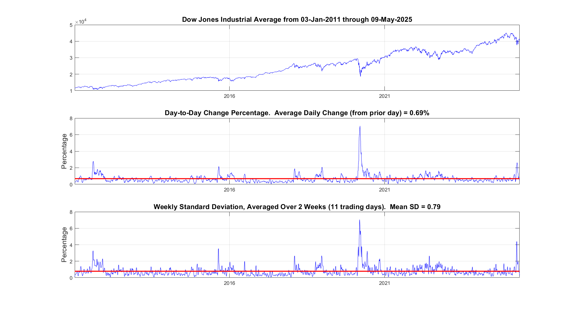
It seems like the financial news is always saying the stock market is especially volatile now. But is it really? This code will show you the daily variation from the prior day. You can see that the average daily change from one day to the next is 0.69%. So any change in the stock market from the prior day less than about 0.7% or 1% is just normal "noise"/typical variation. You can modify the code to adjust the starting date for the analysis. Data file (Excel workbook) is attached (hopefully - I attached it twice but it's not showing up yet).
% Program to plot the Dow Jones Industrial Average from 1928 to May 2025, and compute the standard deviation.
% Data available for download at https://finance.yahoo.com/quote/%5EDJI/history?p=%5EDJI
% Just set the Time Period, then find and click the download link, but you ned a paid version of Yahoo.
%
% If you have a subscription for Microsoft Office 365, you can also get historical stock prices.
% Reference: https://support.microsoft.com/en-us/office/stockhistory-function-1ac8b5b3-5f62-4d94-8ab8-7504ec7239a8#:~:text=The%20STOCKHISTORY%20function%20retrieves%20historical,Microsoft%20365%20Business%20Premium%20subscription.
% For example put this in an Excel Cell
% =STOCKHISTORY("^DJI", "1/1/2000", "5/10/2025", 0, 1, 0, 1,2,3,4, 5)
% and it will fill out a table in Excel
%====================================================================================================================
clc; % Clear the command window.
close all; % Close all figures (except those of imtool.)
imtool close all; % Close all imtool figures if you have the Image Processing Toolbox.
clear; % Erase all existing variables. Or clearvars if you want.
workspace; % Make sure the workspace panel is showing.
format long g;
format compact;
fontSize = 14;
filename = 'Dow Jones Industrial Index.xlsx';
data = readtable(filename);
% Date,Close,Open,High,Low,Volume
dates = data.Date;
closing = data.Close;
volume = data.Volume;
% Define start date and stop date
startDate = datetime(2011,1,1)
stopDate = dates(end)
selectedDates = dates > startDate;
% Extract those dates:
dates = dates(selectedDates);
closing = closing(selectedDates);
volume = volume(selectedDates);
% Plot Volume
hFigVolume = figure('Name', 'Daily Volume');
plot(dates, volume, 'b-');
grid on;
xticks(startDate:calendarDuration(5,0,0):stopDate)
title('Dow Jones Industrial Average Volume', 'FontSize', fontSize);
hFig = figure('Name', 'Daily Standard Deviation');
subplot(3, 1, 1);
plot(dates, closing, 'b-');
xticks(startDate:calendarDuration(5,0,0):stopDate)
drawnow;
grid on;
caption = sprintf('Dow Jones Industrial Average from %s through %s', dates(1), dates(end));
title(caption, 'FontSize', fontSize);
% Get the average change from one trading day to the next.
diffs = 100 * abs(closing(2:end) - closing(1:end-1)) ./ closing(1:end-1);
subplot(3, 1, 2);
averageDailyChange = mean(diffs)
% Looks pretty noisy so let's smooth it for a nicer display.
numWeeks = 4;
diffs = sgolayfilt(diffs, 2, 5*numWeeks+1);
plot(dates(2:end), diffs, 'b-');
grid on;
xticks(startDate:calendarDuration(5,0,0):stopDate)
hold on;
line(xlim, [averageDailyChange, averageDailyChange], 'Color', 'r', 'LineWidth', 2);
ylabel('Percentage', 'FontSize', fontSize);
caption = sprintf('Day-to-Day Change Percentage. Average Daily Change (from prior day) = %.2f%%', averageDailyChange);
title(caption, 'FontSize', fontSize);
drawnow;
% Get the stddev over a 5 trading day window.
sd = stdfilt(closing, ones(5, 1));
% Get it relative to the magnitude.
sd = sd ./ closing * 100;
averageVariation = mean(sd)
numWeeks = 2;
% Looks pretty noisy so let's smooth it for a nicer display.
sd = sgolayfilt(sd, 2, 5*numWeeks+1);
% Plot it.
subplot(3, 1, 3);
plot(dates, sd, 'b-');
grid on;
xticks(startDate:calendarDuration(5,0,0):stopDate)
hold on;
line(xlim, [averageVariation, averageVariation], 'Color', 'r', 'LineWidth', 2);
ylabel('Percentage', 'FontSize', fontSize);
caption = sprintf('Weekly Standard Deviation, Averaged Over %d Weeks (%d trading days). Mean SD = %.2f', ...
numWeeks, 5*numWeeks+1, averageVariation);
title(caption, 'FontSize', fontSize);
% Maximize figure window.
g = gcf;
g.WindowState = 'maximized';
w = logspace(-1,3,100);
[m,p] = bode(tf(1,[1 1]),w);
size(m)
and therefore plotting requires an explicit squeeze (or rehape, or colon)
% semilogx(w,squeeze(db(m)))
Similarly, I'm using page* functions more regularly and am now generating 3D results whereas my old code would generate 2D. For example
x = [1;1];
theta = reshape(0:.1:2*pi,1,1,[]);
Z = [cos(theta), sin(theta);-sin(theta),cos(theta)];
y = pagemtimes(Z,x);
Now, plotting requires squeezing the inputs
% plot(squeeze(theta),squeeze(y))
Would there be any drawbacks to having plot, et. al., automagically apply squeeze to its inputs?