Main Content

Results for

Let S be the closed surface composed of the hemisphere and the base Let be the electric field defined by . Find the electric flux through S. (Hint: Divide S into two parts and calculate ).
% Define the limits of integration for the hemisphere S1
theta_lim = [-pi/2, pi/2];
phi_lim = [0, pi/2];
% Perform the double integration over the spherical surface of the hemisphere S1
% Define the electric flux function for the hemisphere S1
flux_function_S1 = @(theta, phi) 2 * sin(phi);
electric_flux_S1 = integral2(flux_function_S1, theta_lim(1), theta_lim(2), phi_lim(1), phi_lim(2));
% For the base of the hemisphere S2, the electric flux is 0 since the electric
% field has no z-component at the base
electric_flux_S2 = 0;
% Calculate the total electric flux through the closed surface S
total_electric_flux = electric_flux_S1 + electric_flux_S2;
% Display the flux calculations
disp(['Electric flux through the hemisphere S1: ', num2str(electric_flux_S1)]);
disp(['Electric flux through the base of the hemisphere S2: ', num2str(electric_flux_S2)]);
disp(['Total electric flux through the closed surface S: ', num2str(total_electric_flux)]);
% Parameters for the plot
radius = 1; % Radius of the hemisphere
% Create a meshgrid for theta and phi for the plot
[theta, phi] = meshgrid(linspace(theta_lim(1), theta_lim(2), 20), linspace(phi_lim(1), phi_lim(2), 20));
% Calculate Cartesian coordinates for the points on the hemisphere
x = radius * sin(phi) .* cos(theta);
y = radius * sin(phi) .* sin(theta);
z = radius * cos(phi);
% Define the electric field components
Ex = 2 * x;
Ey = 2 * y;
Ez = 2 * z;
% Plot the hemisphere
figure;
surf(x, y, z, 'FaceAlpha', 0.5, 'EdgeColor', 'none');
hold on;
% Plot the electric field vectors
quiver3(x, y, z, Ex, Ey, Ez, 'r');
% Plot the base of the hemisphere
[x_base, y_base] = meshgrid(linspace(-radius, radius, 20), linspace(-radius, radius, 20));
z_base = zeros(size(x_base));
surf(x_base, y_base, z_base, 'FaceColor', 'cyan', 'FaceAlpha', 0.3);
% Additional plot settings
colormap('cool');
axis equal;
grid on;
xlabel('X');
ylabel('Y');
zlabel('Z');
title('Hemisphere and Electric Field');
David
David
Last activity on 2 Apr 2024

I feel like no one at UC San Diego knows this page, let alone this server, is still live. For the younger generation, this is what the whole internet used to look like :)
%%
clear
clc
close all
% TODO - Replace the [] with channel ID to write data to:
writeChannelID = 'your channel ID'; %channel ID
% TODO - Enter the Write API Key between the '' below:
writeAPIKey = 'your write API Key'; %write API Key
% url for POST request
url = 'https://aemo.com.au/';
webText = webread(url);
filteredData(4) = urlfilter(url,'<div class="summary-row-value">');
display(filteredData(4), 'AEMO');
thingSpeakWrite(writeChannelID, filteredData(4), 'WriteKey', writeAPIKey);
Edward
Edward
Last activity on 3 Apr 2024

The cloks have changed in the UK having gone forward 1 hour but the times on the thingspeak graphs are out an hour - what is the solution please
The line integral 
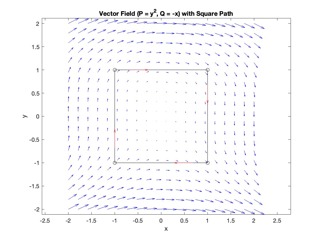
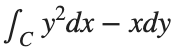
, where C is the boundary of the square
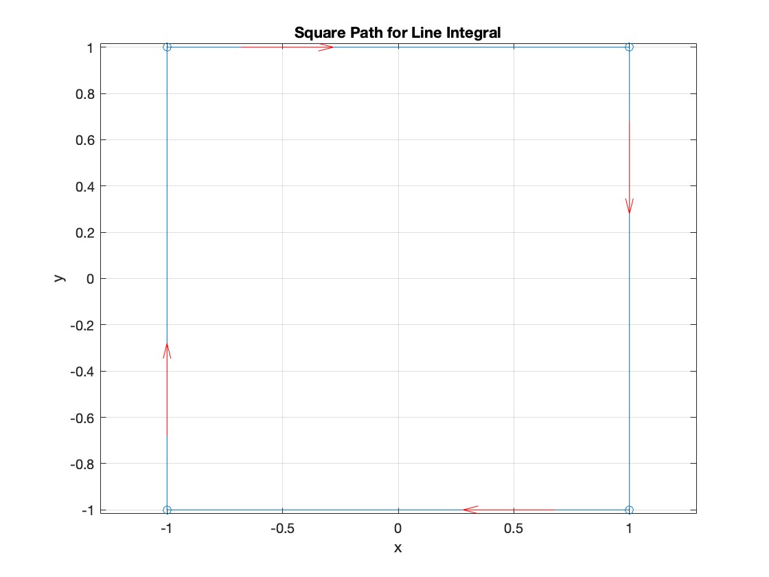
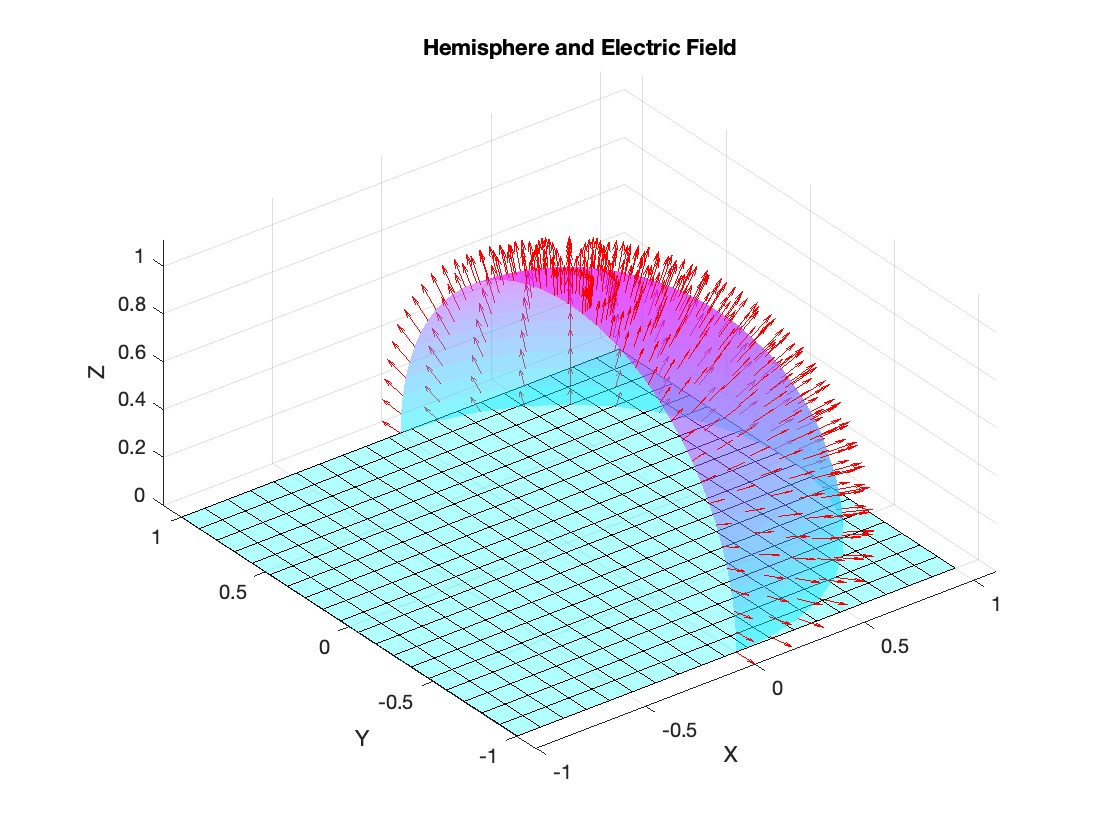
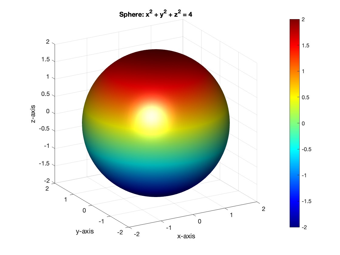
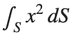
 oriented counterclockwise, can be evaluated in two ways:
Using the definition of the line integral:
% Initialize the integral sum
integral_sum = 0;
% Segment C1: x = -1, y goes from -1 to 1
y = linspace(-1, 1);
x = -1 * ones(size(y));
dy = diff(y);
integral_sum = integral_sum + sum(-x(1:end-1) .* dy);
% Segment C2: y = 1, x goes from -1 to 1
x = linspace(-1, 1);
y = ones(size(x));
dx = diff(x);
integral_sum = integral_sum + sum(y(1:end-1).^2 .* dx);
% Segment C3: x = 1, y goes from 1 to -1
y = linspace(1, -1);
x = ones(size(y));
dy = diff(y);
integral_sum = integral_sum + sum(-x(1:end-1) .* dy);
% Segment C4: y = -1, x goes from 1 to -1
x = linspace(1, -1);
y = -1 * ones(size(x));
dx = diff(x);
integral_sum = integral_sum + sum(y(1:end-1).^2 .* dx);
disp(['Direct Method Integral: ', num2str(integral_sum)]);
Plotting the square path
% Define the square's vertices
vertices = [-1 -1; -1 1; 1 1; 1 -1; -1 -1];
% Plot the square
figure;
plot(vertices(:,1), vertices(:,2), '-o');
title('Square Path for Line Integral');
xlabel('x');
ylabel('y');
grid on;
axis equal;
% Add arrows to indicate the path direction (counterclockwise)
hold on;
for i = 1:size(vertices,1)-1
% Calculate direction
dx = vertices(i+1,1) - vertices(i,1);
dy = vertices(i+1,2) - vertices(i,2);
% Reduce the length of the arrow for better visibility
scale = 0.2;
dx = scale * dx;
dy = scale * dy;
% Calculate the start point of the arrow
startx = vertices(i,1) + (1 - scale) * dx;
starty = vertices(i,2) + (1 - scale) * dy;
% Plot the arrow
quiver(startx, starty, dx, dy, 'MaxHeadSize', 0.5, 'Color', 'r', 'AutoScale', 'off');
end
hold off;
Apply Green's Theorem for the line integral
% Define the partial derivatives of P and Q
f = @(x, y) -1 - 2*y; % derivative of -x with respect to x is -1, and derivative of y^2 with respect to y is 2y
% Compute the double integral over the square [-1,1]x[-1,1]
integral_value = integral2(f, -1, 1, 1, -1);
disp(['Green''s Theorem Integral: ', num2str(integral_value)]);
Plotting the vector field related to Green’s theorem
% Define the grid for the vector field
[x, y] = meshgrid(linspace(-2, 2, 20), linspace(-2 ,2, 20));
% Define the vector field components
P = y.^2; % y^2 component
Q = -x; % -x component
% Plot the vector field
figure;
quiver(x, y, P, Q, 'b');
hold on; % Hold on to plot the square on the same figure
% Define the square's vertices
vertices = [-1 -1; -1 1; 1 1; 1 -1; -1 -1];
% Plot the square path
plot(vertices(:,1), vertices(:,2), '-o', 'Color', 'k'); % 'k' for black color
title('Vector Field (P = y^2, Q = -x) with Square Path');
xlabel('x');
ylabel('y');
axis equal;
% Add arrows to indicate the path direction (counterclockwise)
for i = 1:size(vertices,1)-1
% Calculate direction
dx = vertices(i+1,1) - vertices(i,1);
dy = vertices(i+1,2) - vertices(i,2);
% Reduce the length of the arrow for better visibility
scale = 0.2;
dx = scale * dx;
dy = scale * dy;
% Calculate the start point of the arrow
startx = vertices(i,1) + (1 - scale) * dx;
starty = vertices(i,2) + (1 - scale) * dy;
% Plot the arrow
quiver(startx, starty, dx, dy, 'MaxHeadSize', 0.5, 'Color', 'r', 'AutoScale', 'off');
end
hold off;
To solve a surface integral for example the over the sphere easily in MATLAB, you can leverage the symbolic toolbox for a direct and clear solution. Here is a tip to simplify the process:
  1. Use Symbolic Variables and Functions: Define your variables symbolically, including the parameters of your spherical coordinates θ and ϕ and the radius r . This allows MATLAB to handle the expressions symbolically, making it easier to manipulate and integrate them.
  2. Express in Spherical Coordinates Directly: Since you already know the sphere's equation and the relationship in spherical coordinates, define x, y, and z in terms of r , θ and ϕ directly.
  3. Perform Symbolic Integration: Use MATLAB's `int` function to integrate symbolically. Since the sphere and the function are symmetric, you can exploit these symmetries to simplify the calculation.
Here’s how you can apply this tip in MATLAB code:
% Include the symbolic math toolbox
syms theta phi
% Define the limits for theta and phi
theta_limits = [0, pi];
phi_limits = [0, 2*pi];
% Define the integrand function symbolically
integrand = 16 * sin(theta)^3 * cos(phi)^2;
% Perform the symbolic integral for the surface integral
surface_integral = int(int(integrand, theta, theta_limits(1), theta_limits(2)), phi, phi_limits(1), phi_limits(2));
% Display the result of the surface integral symbolically
disp(['The surface integral of x^2 over the sphere is ', char(surface_integral)]);
% Number of points for plotting
num_points = 100;
% Define theta and phi for the sphere's surface
[theta_mesh, phi_mesh] = meshgrid(linspace(double(theta_limits(1)), double(theta_limits(2)), num_points), ...
linspace(double(phi_limits(1)), double(phi_limits(2)), num_points));
% Spherical to Cartesian conversion for plotting
r = 2; % radius of the sphere
x = r * sin(theta_mesh) .* cos(phi_mesh);
y = r * sin(theta_mesh) .* sin(phi_mesh);
z = r * cos(theta_mesh);
% Plot the sphere
figure;
surf(x, y, z, 'FaceColor', 'interp', 'EdgeColor', 'none');
colormap('jet'); % Color scheme
shading interp; % Smooth shading
camlight headlight; % Add headlight-type lighting
lighting gouraud; % Use Gouraud shading for smooth color transitions
title('Sphere: x^2 + y^2 + z^2 = 4');
xlabel('x-axis');
ylabel('y-axis');
zlabel('z-axis');
colorbar; % Add color bar to indicate height values
axis square; % Maintain aspect ratio to be square
view([-30, 20]); % Set a nice viewing angle
I am often talking to new MATLAB users. I have put together one script. If you know how this script works, why, and what each line means, you will be well on your way on your MATLAB learning journey.
% Clear existing variables and close figures
clear;
close all;
% Print to the Command Window
disp('Hello, welcome to MATLAB!');
% Create a simple vector and matrix
vector = [1, 2, 3, 4, 5];
matrix = [1, 2, 3; 4, 5, 6; 7, 8, 9];
% Display the created vector and matrix
disp('Created vector:');
disp(vector);
disp('Created matrix:');
disp(matrix);
% Perform element-wise multiplication
result = vector .* 2;
% Display the result of the operation
disp('Result of element-wise multiplication of the vector by 2:');
disp(result);
% Create plot
x = 0:0.1:2*pi; % Generate values from 0 to 2*pi
y = sin(x); % Calculate the sine of these values
% Plotting
figure; % Create a new figure window
plot(x, y); % Plot x vs. y
title('Simple Plot of sin(x)'); % Give the plot a title
xlabel('x'); % Label the x-axis
ylabel('sin(x)'); % Label the y-axis
grid on; % Turn on the grid
disp('This is the end of the script. Explore MATLAB further to learn more!');
Hannah
Hannah
Last activity on 1 Apr 2024

Although, I think I will only get to see a partial eclipse (April 8th!) from where I am at in the U.S. I will always have MATLAB to make my own solar eclipse. Just as good as the real thing.
Code (found on the @MATLAB instagram)
a=716;
v=255;
X=linspace(-10,10,a);
[~,r]=cart2pol(X,X');
colormap(gray.*[1 .78 .3]);
[t,g]=cart2pol(X+2.6,X'+1.4);
image(rescale(-1*(2*sin(t*10)+60*g.^.2),0,v))
hold on
h=exp(-(r-3)).*abs(ifft2(r.^-1.8.*cos(7*rand(a))));
h(r<3)=0;
image(v*ones(a),'AlphaData',rescale(h,0,1))
camva(3.8)
Gabriel
Gabriel
Last activity on 29 Mar 2024

I keep getting this error, what do I do?
Error: File: convert_mnist_to_mat.m Line: 63 Column: 1
This statement is not inside any function.
(It follows the END that terminates the definition of the function
"read_mnist_labels".)
function convert_mnist_to_mat(mnist_dir, output_file)
% Function to convert MNIST dataset files into .mat format
% Check if the directory exists
if ~isfolder(mnist_dir)
error('MNIST directory does not exist.');
end
% Read training images
train_images = read_mnist_images(fullfile(mnist_dir, 'train-images-idx3-ubyte'));
% Read training labels
train_labels = read_mnist_labels(fullfile(mnist_dir, 'train-labels-idx1-ubyte'));
% Read test images
test_images = read_mnist_images(fullfile(mnist_dir, 't10k-images-idx3-ubyte'));
% Read test labels
test_labels = read_mnist_labels(fullfile(mnist_dir, 't10k-labels-idx1-ubyte'));
% Save data into .mat file
save(output_file, 'train_images', 'train_labels', 'test_images', 'test_labels');
disp('MNIST dataset converted successfully.');
end
function images = read_mnist_images(filename)
% Function to read MNIST image data
fid = fopen(filename, 'rb');
assert(fid ~= -1, ['Could not open ', filename, '']);
magic_number = fread(fid, 1, 'int32', 0, 'ieee-be');
assert(magic_number == 2051, ['Invalid magic number in ', filename]);
num_images = fread(fid, 1, 'int32', 0, 'ieee-be');
num_rows = fread(fid, 1, 'int32', 0, 'ieee-be');
num_cols = fread(fid, 1, 'int32', 0, 'ieee-be');
images = fread(fid, [num_rows, num_cols, num_images], 'uint8');
fclose(fid);
images = permute(images, [2, 1, 3]); % Convert from (rows, cols, images) to (cols, rows, images)
end
function labels = read_mnist_labels(filename)
% Function to read MNIST label data
fid = fopen(filename, 'rb');
assert(fid ~= -1, ['Could not open ', filename, '']);
magic_number = fread(fid, 1, 'int32', 0, 'ieee-be');
assert(magic_number == 2049, ['Invalid magic number in ', filename]);
num_labels = fread(fid, 1, 'int32', 0, 'ieee-be');
labels = fread(fid, [num_labels, 1], 'uint8');
fclose(fid);
end
% Usage example:
mnist_dir = 'C:\Users\gabep\Desktop\MNIST';
output_file = 'mnist_dataset.mat';
convert_mnist_to_mat(mnist_dir, output_file);
One of the privileges of working at MathWorks is that I get to hang out with some really amazing people. Steve Eddins, of ‘Steve on Image Processing’ fame is one of those people. He recently announced his retirement and before his final day, I got the chance to interview him. See what he had to say over at The MATLAB Blog The Steve Eddins Interview: 30 years of MathWorking
Hi everyone, I need help for transfering the data from a ThingSpeak' channel to Google Sheets. Please help me.
Hassan Ali
Hassan Ali
Last activity on 25 May 2024

Hello everyone.
I have modelled a three phase inverter to run a 5Kw PMSM motor (MATLAB preparametrized). The torque load is applied through ideal torque source and step junction, and the speed of the motor is visualized. When I provide the gate signal only through SPWM generator (No control, only SPWM signal generation through carrier and sine wave comparison),
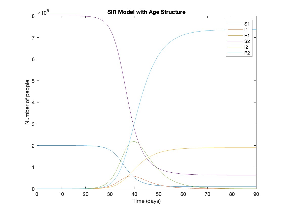
  • The speed stabilizes around 62 rad/sec after some initial oscillations, but when I try to run the same model using PMSM field oriented control block set, the speed is negative (negative rotation) and it keeps on increasing eventhough the speed reference provided is only upto 60. The waveform of both speed and torque has been attached hereby.
  • Moreover, is there anyway to tune the PI controllers (inner and outer loops) of PMSM Field oriented blockset automatically.
  • It can be seen from the torque waveform, there is soemkind of disturbance around 0.4-0.45 sec, which creates too much noise in current, torque waveforms. What could be the reason behind this.
Your help would be highly appreciated.
Thank you.
Before we begin, you will need to make sure you have 'sir_age_model.m' installed. Once you've downloaded this folder into your working directory, which can be located at your current folder. If you can see this file in your current folder, then it's safe to use it. If you choose to use MATLAB online or MATLAB Mobile, you may upload this to your MATLAB Drive.
This is the code for the SIR model stratified into 2 age groups (children and adults). For a detailed explanation of how to derive the force of infection by age group.
% Main script to run the SIR model simulation
% Initial state values
initial_state_values = [200000; 1; 0; 800000; 0; 0]; % [S1; I1; R1; S2; I2; R2]
% Parameters
parameters = [0.05; 7; 6; 1; 10; 1/5]; % [b; c_11; c_12; c_21; c_22; gamma]
% Time span for the simulation (3 months, with daily steps)
tspan = [0 90];
% Solve the ODE
[t, y] = ode45(@(t, y) sir_age_model(t, y, parameters), tspan, initial_state_values);
% Plotting the results
plot(t, y);
xlabel('Time (days)');
ylabel('Number of people');
legend('S1', 'I1', 'R1', 'S2', 'I2', 'R2');
title('SIR Model with Age Structure');
What was the cumulative incidence of infection during this epidemic? What proportion of those infections occurred in children?
In the SIR model, the cumulative incidence of infection is simply the decline in susceptibility.
% Assuming 'y' contains the simulation results from the ode45 function
% and 't' contains the time points
% Total cumulative incidence
total_cumulative_incidence = (y(1,1) - y(end,1)) + (y(1,4) - y(end,4));
fprintf('Total cumulative incidence: %f\n', total_cumulative_incidence);
% Cumulative incidence in children
cumulative_incidence_children = (y(1,1) - y(end,1));
% Proportion of infections in children
proportion_infections_children = cumulative_incidence_children / total_cumulative_incidence;
fprintf('Proportion of infections in children: %f\n', proportion_infections_children);
927,447 people became infected during this epidemic, 20.5% of which were children.
Which age group was most affected by the epidemic?
To answer this, we can calculate the proportion of children and adults that became infected.
% Assuming 'y' contains the simulation results from the ode45 function
% and 't' contains the time points
% Proportion of children that became infected
initial_children = 200000; % initial number of susceptible children
final_susceptible_children = y(end,1); % final number of susceptible children
proportion_infected_children = (initial_children - final_susceptible_children) / initial_children;
fprintf('Proportion of children that became infected: %f\n', proportion_infected_children);
% Proportion of adults that became infected
initial_adults = 800000; % initial number of susceptible adults
final_susceptible_adults = y(end,4); % final number of susceptible adults
proportion_infected_adults = (initial_adults - final_susceptible_adults) / initial_adults;
fprintf('Proportion of adults that became infected: %f\n', proportion_infected_adults);
Throughout this epidemic, 95% of all children and 92% of all adults were infected. Children were therefore slightly more affected in proportion to their population size, even though the majority of infections occurred in adults.
Suppose I want to use tiledlayout to draw a 4*6 figure. Now I want to let the first and second row of figures share the same ylabels, and so do the third and the fourth. But I did not find a way to do this. I tried to create two different tiledlayout on one figure, but tiledlayout did not allow me to do so. Thus, any suggestions?
Are you going to be in the path of totality? How can you predict, track, and simulate the solar eclipse using MATLAB?

Englisch Translate Französisch Deutsch Deutsch Russisch PONS Deepl übersetzer Spanisch Deutsch DeepL kostenlos Deutsch Englisch hallo, ich bitte um Hilfe! Seit Jahren habe ich Konto auf Thingspeak, den ich für meinen Zweck nicht richtig nutzen kann. Ich kann "Upoad to meine private Chanel", aber das lesen funktioniert nicht, weder in ArdunioIDE, noch Ardunio iot kann ich die gesendete Daten (Temperatur) von einem anderen Board lesen, es ist egal, ob ESP8266, ESP32, MKR, oder UnoWifi Rev2. Nichts! Die Beispiele im Bibliotek sind eine Katastrophe, "wetter-chanel" und diese funktionieren auch nicht. Auch nicht die von GitHub. Es sollte aber einfach sein, denn auf meiner Seite sehe ich ja "GET"+ url. inkl json+result.

Wo gibt es eine richtige sketch für "read private chanel/field" , welche funktioniert? Man braucht nicht die Wifi-Enstellungen, sondern den code für die Abfrage, "Serial.print"(value)"

Bitte um Hilfe, danke schön.

hello, I ask for help! I've had an account on Thingspeak for years, but I can't use it properly for my purpose. I can "Upoad to my private Chanel", but reading doesn't work, neither in ArdunioIDE nor Ardunio iot can I read the sent data (temperature) from another board, it doesn't matter whether ESP8266, ESP32, MKR, or UnoWifi Rev2. Nothing! The examples in the library are a disaster, "weather-chanel" and they don't work either. Not even the one from GitHub. But it should be easy, because on my site I see “GET”+ url. including json+result.

Where is there a proper sketch for "read private chanel/field" that works? You don't need the WiFi settings, but the code for the query, "Serial.print"(value)"

Please help, thank you very much.

Hello Everyone,
I'm running an IoT project at my university using a free . Basically, my system uploads the sensor data to 4 different fields of a ThingSpeak channel and I'm reading from or writing to the channel through Simulink. I have a few questions regarding this topic:
  1. I'm trying to upload to the server every 3 seconds (which seemed to be providing the best results so far). Since the channel only accepts data transmit every 15 seconds, what is the optimized upload interval rate to match the interval rate of the channel? Because otherwise I have realized that my interval rate can go up to 1min sometimes for some reason.
  2. Is reading from/writing to the channel through simulink while the system is uploading data to the channel slow down th whole process? What is your overall suggestion in this case?
I'm excited to hear your suggestions and experiences!
Regards,
Ege
Product Models:LPS8N dragino
Firmware Version: lgw--build-v5.4.1704801796-20240109-2005
Hi all
at the moment i can not work with CODE dragino lora to gateway LPS8N and MQTT thingSpeak.
with root commands i can send DATA to thingspeak
mosquito_pub -d -h mqtt3.thingspeak.com -p 1883 -u PSoyJxYWBTQ9Hx8cExMZ... -I PSoyJxYWBTQ9Hx8cExM.... -P hCEd77jdiziYzUV6ygl.... -t channels/2466703/publish -m “field1=100&field2=100&status=MQTTPUBLISH”
so my question there anybody that can work with LPS8N dragino to MQTT ThingSpeak? which code arduino are using?
thanks in advance to answer.
Nelson
The latest release is pretty much upon us. Official annoucements will be coming soon and the eagle-eyed among you will have started to notice some things shifting around on the MathWorks website as we ready for this.
The pre-release has been available for a while. Maybe you've played with it? I have...I've even been quietly using it to write some of my latest blog posts...and I have several queued up for publication after MathWorks officially drops the release.
At the time of writing, this page points to the pre-release highlights. Prerelease Release Highlights - MATLAB & Simulink (mathworks.com)
What excites you about this release? why?
The stationary solutions of the Klein-Gordon equation refer to solutions that are time-independent, meaning they remain constant over time. For the non-linear Klein-Gordon equation you are discussing:
Stationary solutions arise when the time derivative term, 
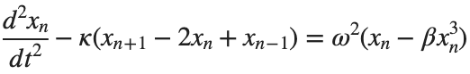
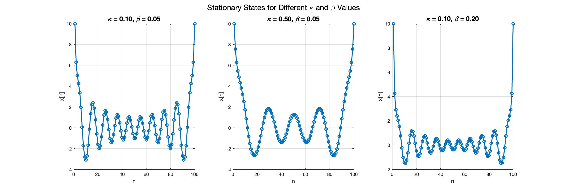
, is zero, meaning the motion of the system does not change over time. This leads to a static differential equation:
This equation describes how particles in the lattice interact with each other and how non-linearity affects the steady state of the system.
The solutions to this equation correspond to the various possible stable equilibrium states of the system, where each represents different static distribution patterns of displacements . The specific form of these stationary solutions depends on the system parameters, such as κ , ω, and β , as well as the initial and boundary conditions of the problem.
To find these solutions in a more specific form, one might need to solve the equation using analytical or numerical methods, considering the different cases that could arise in such a non-linear system.
By interpreting the equation in this way, we can relate the dynamics described by the discrete Klein - Gordon equation to the behavior of DNA molecules within a biological system . This analogy allows us to understand the behavior of DNA in terms of concepts from physics and mathematical modeling .
% Parameters
numBases = 100; % Number of spatial points
omegaD = 0.2; % Common parameter for the equation
% Preallocate the array for the function handles
equations = cell(numBases, 1);
% Initial guess for the solution
initialGuess = 0.01 * ones(numBases, 1);
% Parameter sets for kappa and beta
paramSets = [0.1, 0.05; 0.5, 0.05; 0.1, 0.2];
% Prepare figure for subplot
figure;
set(gcf, 'Position', [100, 100, 1200, 400]); % Set figure size
% Newton-Raphson method parameters
maxIterations = 1000;
tolerance = 1e-10;
% Set options for fsolve to use the 'levenberg-marquardt' algorithm
options = optimoptions('fsolve', 'Algorithm', 'levenberg-marquardt', 'MaxIterations', maxIterations, 'FunctionTolerance', tolerance);
for i = 1:size(paramSets, 1)
kappa = paramSets(i, 1);
beta = paramSets(i, 2);
% Define the equations using a function
for n = 2:numBases-1
equations{n} = @(x) -kappa * (x(n+1) - 2 * x(n) + x(n-1)) - omegaD^2 * (x(n) - beta * x(n)^3);
end
% Boundary conditions with specified fixed values
someFixedValue1 = 10; % Replace with actual value if needed
someFixedValue2 = 10; % Replace with actual value if needed
equations{1} = @(x) x(1) - someFixedValue1;
equations{numBases} = @(x) x(numBases) - someFixedValue2;
% Combine all equations into a single function
F = @(x) cell2mat(cellfun(@(f) f(x), equations, 'UniformOutput', false));
% Solve the system of equations using fsolve with the specified options
x_solution = fsolve(F, initialGuess, options);
norm(F(x_solution))
% Plot the solution in a subplot
subplot(1, 3, i);
plot(x_solution, 'o-', 'LineWidth', 2);
grid on;
xlabel('n', 'FontSize', 12);
ylabel('x[n]', 'FontSize', 12);
title(sprintf('\\kappa = %.2f, \\beta = %.2f', kappa, beta), 'FontSize', 14);
end
% Improve overall aesthetics
sgtitle('Stationary States for Different \kappa and \beta Values', 'FontSize', 16); % Super title for the figure
In the second plot, the elasticity constant κis increased to 0.5, representing a system with greater stiffness . This parameter influences how resistant the system is to deformation, implying that a higher κ makes the system more resilient to changes . By increasing κ, we are essentially tightening the interactions between adjacent units in the model, which could represent, for instance, stronger bonding forces in a physical or biological system .
In the third plot the nonlinearity coefficient β is increased to 0.2 . This adjustment enhances the nonlinear interactions within the system, which can lead to more complex dynamic behaviors, especially in systems exhibiting bifurcations or chaos under certain conditions .