Results for
Problem statement: I've written a visualization that I'd like to use on potentially hundreds of different channels in my commerical account. Because it contains code that's unique to the channel (channel id, read API key, etc.) I have to create and maintain a duplicate visualization for each channel. This is wasteful, a source of errors, and almost intractable for a commercial customer with a high channel count.
My request is that MATLAB Visualizations be extended to support parameters, but only a predefined set to reduce the scope. I would propose a subset of the parameters currently supported by the ThingSpeak API. For example, thingSpeakRead supports (requires) readChannelID, NumPoints, and a ReadKey etc. If those were elevated to also be allowed as Visualization parameters, I imagine it would satisfy a large subset of user needs.
The poor man's version of this would be if ThingSpeak supported just one special parameter, such as %CHANNEL_ID%. If this was available within the visualization code one could use it as a key into table to get the other pieces of data like API keys, etc. It would be have to be passed on the visualization url (https://thingspeak.com/apps/matlab_visualizations/573779?readChannelID=xxxxx). Not sure how the visualization would pick it up in the use case where it's called from the ThingSpeak website under the user's list of MATLAB Visualizations. Perhaps it can be prompted for.
I initially considered user defined functions or libraries but they are not supported and I can see that that would require even more development work to support. The workarounds described in this thread aren't suitable for me. https://www.mathworks.com/matlabcentral/answers/2102981-how-to-use-private-functions-lib-in-thingspeak?s_tid=srchtitle_community_thingspeak_14_libraries
thanks!
Tom
Hello everyone, i hope you all are in good health. i need to ask you about the help about where i should start to get indulge in matlab. I am an electrical engineer but having experience of construction field. I am new here. Please do help me. I shall be waiting forward to hear from you. I shall be grateful to you. Need recommendations and suggestions from experienced members. Thank you.
I recently wrote up a document which addresses the solution of ordinary and partial differential equations in Matlab (with some Python examples thrown in for those who are interested). For ODEs, both initial and boundary value problems are addressed. For PDEs, it addresses parabolic and elliptic equations. The emphasis is on finite difference approaches and built-in functions are discussed when available. Theory is kept to a minimum. I also provide a discussion of strategies for checking the results, because I think many students are too quick to trust their solutions. For anyone interested, the document can be found at https://blanchard.neep.wisc.edu/SolvingDifferentialEquationsWithMatlab.pdf
hello i'm working on simulation using simulink which is my title is ENHANCING BATTERYENERGY STORAGE SYSTEMSTHROUGH MODULAR MULTILEVEL CONVERTER WITH STATE-OF-CHARGE BALANCING CONTROL. i already build 9 level mmc. but i dont have any idea for state of charge balancing control.please any suggestion and explain.
how can I link a chinese flow meter to this website
Kindly link me to the Channel Modeling Group.
I read and compreheneded a paper on channel modeling "An Adaptive Geometry-Based Stochastic Model for Non-Isotropic MIMO Mobile-to-Mobile Channels" except the graphical results obtained from the MATLAB codes. I have tried to replicate the same graphs but to no avail from my codes. And I am really interested in the topic, i have even written to the authors of the paper but as usual, there is no reply from them. Kindly assist if possible.
Hi, I'm looking for sites where I can find coding & algorithms problems and their solutions. I'm doing this workshop in college and I'll need some problems to go over with the students and explain how Matlab works by solving the problems with them and then reviewing and going over different solution options. Does anyone know a website like that? I've tried looking in the Matlab Cody By Mathworks, but didn't exactly find what I'm looking for. Thanks in advance.
Die Anzeige der Werte in den einzelnen Feldern ist nicht aktuell.
So werden z.B. um 18:00 Uhr nur die Werte bis 14:00 Uhr angezeigt, auch das verändern des Zeitfensters bringt keine Abhilfe.
Hat jemand eine Idee wie ich die der Uhrzeit ensprechenden Werte zur Anzeige bringe.
Die Werte werden von Shellies und BitShake kontinuierlich übertragen.
My thingSpeak channel kept on updateing the same signal as early eventhough my simulink have update the new signal. How to solve this?
Any one have deep learning reinforcement based speed control of induction motor?
Hi ThingSpeak Community,
I hope you are all doing well.
I am currently setting up a Vodafone ACL for a SIM card that will be used in a device destined for a remote charity deployment in a week. The goal is to ensure that the device can reliably upload data to ThingSpeak without any connectivity issues.
Here are the details of my current ACL setup:
- FQDN: api.thingspeak.com (specified as the API endpoint)
- IPv4 Address: 184.106.153.149 (found online)
- Port: (left empty)
I've attached a photo of the setup for reference.
Could you please confirm if the above ACL settings are correct? Additionally, if there are any other considerations or settings I should be aware of for ensuring reliable connectivity with ThingSpeak, I would greatly appreciate your guidance.
Currently, all I am using for the device credentials is the PIN number. Do I need to adjust any settings in the Arduino code or the ACL to maintain stable connectivity with ThingSpeak, especially considering the device will be in a remote location and difficult to access for adjustments?
Your prompt assistance and advice will be immensely valuable, as I want to ensure everything is correctly configured before deployment.
Thank you very much!
Best regards,
Arthur
错误使用 ipqpdense
The interior convex algorithm requires all objective and constraint values to be finite.
出错 quadprog
ipqpdense(full(H), f, A, B, Aeq, Beq, lb, ub, X0, flags, ...
出错 MPC_maikenamulun
[X, fval,exitflag]=quadprog(H,f,A_cons,B_cons,[],[],lb,ub,[],options);
Hello, everyone! I’m Mark Hayworth, but you might know me better in the community as Image Analyst. I've been using MATLAB since 2006 (18 years). My background spans a rich career as a former senior scientist and inventor at The Procter & Gamble Company (HQ in Cincinnati). I hold both master’s & Ph.D. degrees in optical sciences from the College of Optical Sciences at the University of Arizona, specializing in imaging, image processing, and image analysis. I have 40+ years of military, academic, and industrial experience with image analysis programming and algorithm development. I have experience designing custom light booths and other imaging systems. I also work with color and monochrome imaging, video analysis, thermal, ultraviolet, hyperspectral, CT, MRI, radiography, profilometry, microscopy, NIR, and Raman spectroscopy, etc. on a huge variety of subjects.
I'm thrilled to participate in MATLAB Central's Ask Me Anything (AMA) session, a fantastic platform for knowledge sharing and community engagement. Following Adam Danz’s insightful AMA on staff contributors in the Answers forum, I’d like to discuss topics in the area of image analysis and processing. I invite you to ask me anything related to this field, whether you're seeking recommendations on tools, looking for tips and tricks, my background, or career development advice. Additionally, I'm more than willing to share insights from my experiences in the MATLAB Answers community, File Exchange, and my role as a member of the Community Advisory Board. If you have questions related to your specific images or your custom MATLAB code though, I'll invite you to ask those in the Answers forum. It's a more appropriate forum for those kinds of questions, plus you can get the benefit of other experts offering their solutions in addition to me.
For the coming weeks, I'll be here to engage with your questions and help shed light on any topics you're curious about.
Hello, everyone!
Over the past few weeks, our community has been buzzing with activity, showcasing the incredible depth of knowledge, creativity, and innovation that makes this forum such a vibrant place. Today, we're excited to highlight some of the noteworthy contributions that have sparked discussions, offered insights, and shared knowledge across various topics. Let's dive in!
Interesting Questions
Fatima Majeed brings us a thought-provoking mathematical challenge, delving into inequalities and the realms beyond (e^e). If you're up for a mathematical journey, this question is a must-see!
lil brain tackles a practical problem many of us have faced: efficiently segmenting a CSV file based on specific criteria. This post is not only a query but a learning opportunity for anyone dealing with similar data manipulation challenges.
Popular Discussions
Discover a simple yet effective trick for digit manipulation from goc3. This tip is especially handy for those frequenting Cody challenges or anyone interested in enhancing their number handling skills in MATLAB.
Chen Lin shares an exciting update about the 'Run Code' feature in the Discussions area, highlighting how our community can now directly execute and share code snippets within discussions. This feature marks a significant enhancement in how we interact and solve problems together.
From the Blogs
A Deep Dive into EEG Analysis for Predicting Neurological Outcomes By Tanya Kuruvilla
Connell D`Souza, alongside Team Swarthbeat, explores the cutting-edge application of EEG analysis in predicting neurological outcomes post-cardiac arrest. This blog post offers an in-depth look into the challenges and methodologies of modern medical data analysis.
Mihir Acharya discusses the pivotal role of MATLAB and Simulink in the future of robotics simulation. Through an engaging conversation with industry analyst George Chowdhury, this post sheds light on overcoming simulation challenges and the exciting possibilities that lie ahead.
We encourage everyone to explore these contributions further and engage with the authors and the community. Your participation is what fuels this community's continual growth and innovation.
Here's to many more discussions, discoveries, and breakthroughs together!
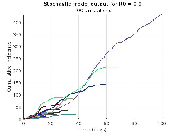
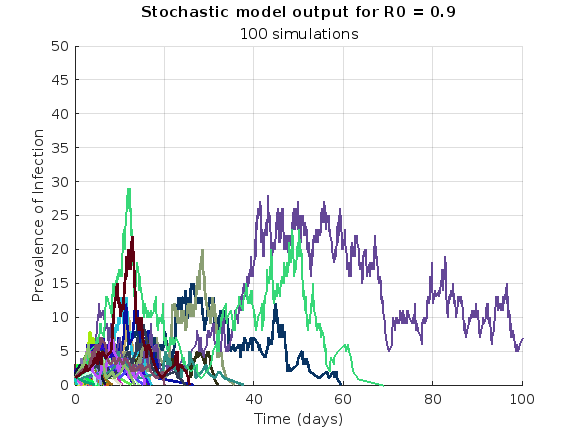
We are modeling the introduction of a novel pathogen into a completely susceptible population. In the cells below, I have provided you with the Matlab code for a simple stochastic SIR model, implemented using the "GillespieSSA" function
Simulating the stochastic model 100 times for 
Since γ is 0.4 per day,  per day
% Define the parameters
beta = 0.36;
gamma = 0.4;
n_sims = 100;
tf = 100; % Time frame changed to 100
% Calculate R0
R0 = beta / gamma
% Initial state values
initial_state_values = [1000000; 1; 0; 0]; % S, I, R, cum_inc
% Define the propensities and state change matrix
a = @(state) [beta * state(1) * state(2) / 1000000, gamma * state(2)];
nu = [-1, 0; 1, -1; 0, 1; 0, 0];
% Define the Gillespie algorithm function
function [t_values, state_values] = gillespie_ssa(initial_state, a, nu, tf)
t = 0;
state = initial_state(:); % Ensure state is a column vector
t_values = t;
state_values = state';
while t < tf
rates = a(state);
rate_sum = sum(rates);
if rate_sum == 0
break;
end
tau = -log(rand) / rate_sum;
t = t + tau;
r = rand * rate_sum;
cum_sum_rates = cumsum(rates);
reaction_index = find(cum_sum_rates >= r, 1);
state = state + nu(:, reaction_index);
% Update cumulative incidence if infection occurred
if reaction_index == 1
state(4) = state(4) + 1; % Increment cumulative incidence
end
t_values = [t_values; t];
state_values = [state_values; state'];
end
end
% Function to simulate the stochastic model multiple times and plot results
function simulate_stoch_model(beta, gamma, n_sims, tf, initial_state_values, R0, plot_type)
% Define the propensities and state change matrix
a = @(state) [beta * state(1) * state(2) / 1000000, gamma * state(2)];
nu = [-1, 0; 1, -1; 0, 1; 0, 0];
% Set random seed for reproducibility
rng(11);
% Initialize plot
figure;
hold on;
for i = 1:n_sims
[t, output] = gillespie_ssa(initial_state_values, a, nu, tf);
% Check if the simulation had only one step and re-run if necessary
while length(t) == 1
[t, output] = gillespie_ssa(initial_state_values, a, nu, tf);
end
if strcmp(plot_type, 'cumulative_incidence')
plot(t, output(:, 4), 'LineWidth', 2, 'Color', rand(1, 3));
elseif strcmp(plot_type, 'prevalence')
plot(t, output(:, 2), 'LineWidth', 2, 'Color', rand(1, 3));
end
end
xlabel('Time (days)');
if strcmp(plot_type, 'cumulative_incidence')
ylabel('Cumulative Incidence');
ylim([0 inf]);
elseif strcmp(plot_type, 'prevalence')
ylabel('Prevalence of Infection');
ylim([0 50]);
end
title(['Stochastic model output for R0 = ', num2str(R0)]);
subtitle([num2str(n_sims), ' simulations']);
xlim([0 tf]);
grid on;
hold off;
end
% Simulate the model 100 times and plot cumulative incidence
simulate_stoch_model(beta, gamma, n_sims, tf, initial_state_values, R0, 'cumulative_incidence');
% Simulate the model 100 times and plot prevalence
simulate_stoch_model(beta, gamma, n_sims, tf, initial_state_values, R0, 'prevalence');
Base case:
Suppose you need to do a computation many times. We are going to assume that this computation cannot be vectorized. The simplest case is to use a for loop:
number_of_elements = 1e6;
test_fcn = @(x) sqrt(x) / x;
tic
for i = 1:number_of_elements
x(i) = test_fcn(i);
end
t_forward = toc;
disp(t_forward + " seconds")
Preallocation:
This can easily be sped up by preallocating the variable that houses results:
tic
x = zeros(number_of_elements, 1);
for i = 1:number_of_elements
x(i) = test_fcn(i);
end
t_forward_prealloc = toc;
disp(t_forward_prealloc + " seconds")
In this example, preallocation speeds up the loop by a factor of about three to four (running in R2024a). Comment below if you get dramatically different results.
disp(sprintf("%.1f", t_forward / t_forward_prealloc))
Run it in reverse:
Is there a way to skip the explicit preallocation and still be fast? Indeed, there is.
clear x
tic
for i = number_of_elements:-1:1
x(i) = test_fcn(i);
end
t_backward = toc;
disp(t_backward + " seconds")
By running the loop backwards, the preallocation is implicitly performed during the first iteration and the loop runs in about the same time (within statistical noise):
disp(sprintf("%.2f", t_forward_prealloc / t_backward))
Do you get similar results when running this code? Let us know your thoughts in the comments below.
Beneficial side effect:
Have you ever had to use a for loop to delete elements from a vector? If so, keeping track of index offsets can be tricky, as deleting any element shifts all those that come after. By running the for loop in reverse, you don't need to worry about index offsets while deleting elements.
We're thrilled to share an exciting update with our community: the 'Run Code' feature is now available in the Discussions area!
Simply insert your code into the editor and press the green triangle button to run it. Your code will execute using the latest MATLAB R24a version, and it supports most common toolboxes. Moreover, this innovative feature allows for the running of attached files, further enhancing its utility and flexibility.
The ‘run code’ feature was first introduced in MATLAB Answers. Encouraged by the positive feedback and at the request of our community members, we are now expanding the availability of this feature to more areas within our community.
As always, your feedback is crucial to us, so please don't hesitate to share your thoughts and experiences by leaving a comment.
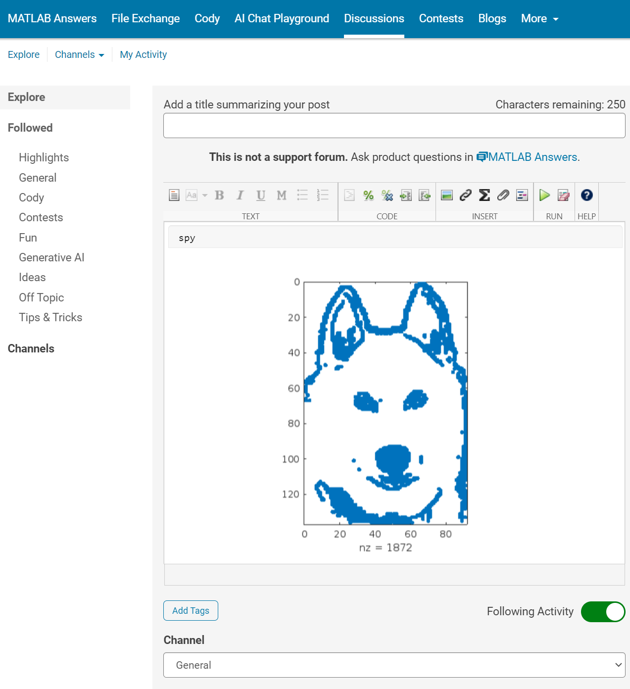
Many times when ploting, we not only need to set the color of the plot, but also its
transparency, Then how we set the alphaData of colorbar at the same time ?
It seems easy to do so :
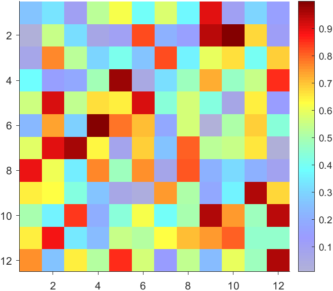
data = rand(12,12);
% Transparency range 0-1, .3-1 for better appearance here
AData = rescale(- data, .3, 1);
% Draw an imagesc with numerical control over colormap and transparency
imagesc(data, 'AlphaData',AData);
colormap(jet);
ax = gca;
ax.DataAspectRatio = [1,1,1];
ax.TickDir = 'out';
ax.Box = 'off';
% get colorbar object
CBarHdl = colorbar;
pause(1e-16)
% Modify the transparency of the colorbar
CData = CBarHdl.Face.Texture.CData;
ALim = [min(min(AData)), max(max(AData))];
CData(4,:) = uint8(255.*rescale(1:size(CData, 2), ALim(1), ALim(2)));
CBarHdl.Face.Texture.ColorType = 'TrueColorAlpha';
CBarHdl.Face.Texture.CData = CData;
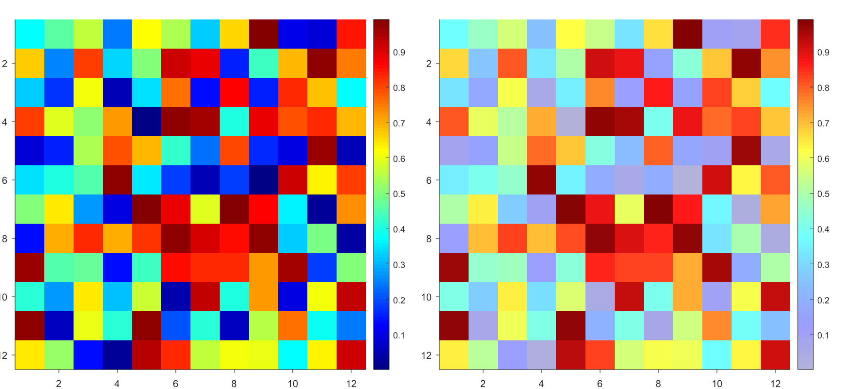
But !!!!!!!!!!!!!!! We cannot preserve the changes when saving them as images :
It seems that when saving plots, the `Texture` will be refresh, but the `Face` will not :
however, object Face only have 4 colors to change(The four corners of a quadrilateral), how
can we set more colors ??
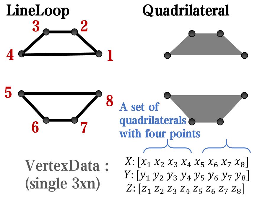
`Face` is a quadrilateral object, and we can change the `VertexData` to draw more than one little quadrilaterals:
data = rand(12,12);
% Transparency range 0-1, .3-1 for better appearance here
AData = rescale(- data, .3, 1);
%Draw an imagesc with numerical control over colormap and transparency
imagesc(data, 'AlphaData',AData);
colormap(jet);
ax = gca;
ax.DataAspectRatio = [1,1,1];
ax.TickDir = 'out';
ax.Box = 'off';
% get colorbar object
CBarHdl = colorbar;
pause(1e-16)
% Modify the transparency of the colorbar
CData = CBarHdl.Face.Texture.CData;
ALim = [min(min(AData)), max(max(AData))];
CData(4,:) = uint8(255.*rescale(1:size(CData, 2), ALim(1), ALim(2)));
warning off
CBarHdl.Face.ColorType = 'TrueColorAlpha';
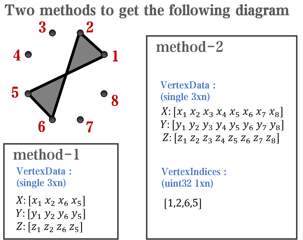
VertexData = CBarHdl.Face.VertexData;
tY = repmat((1:size(CData,2))./size(CData,2), [4,1]);
tY1 = tY(:).'; tY2 = tY - tY(1,1); tY2(3:4,:) = 0; tY2 = tY2(:).';
tM1 = [tY1.*0 + 1; tY1; tY1.*0 + 1];
tM2 = [tY1.*0; tY2; tY1.*0];
CBarHdl.Face.VertexData = repmat(VertexData, [1,size(CData,2)]).*tM1 + tM2;
CBarHdl.Face.ColorData = reshape(repmat(CData, [4,1]), 4, []);
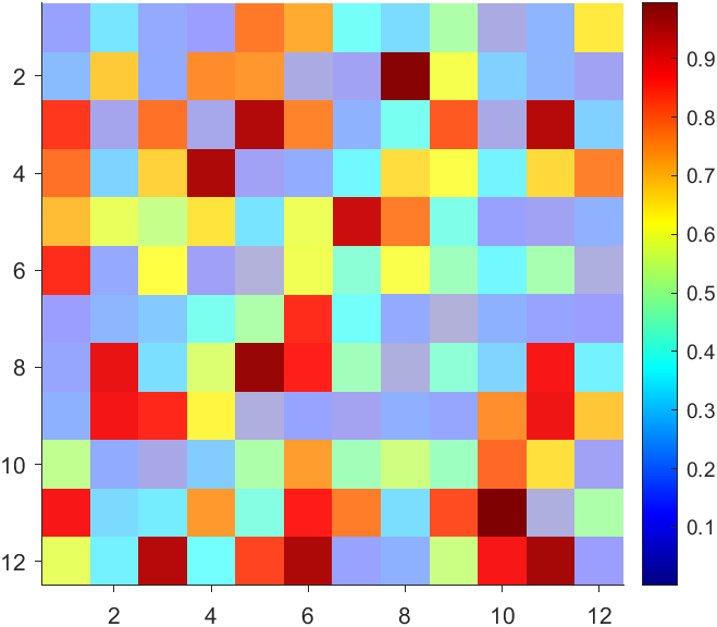
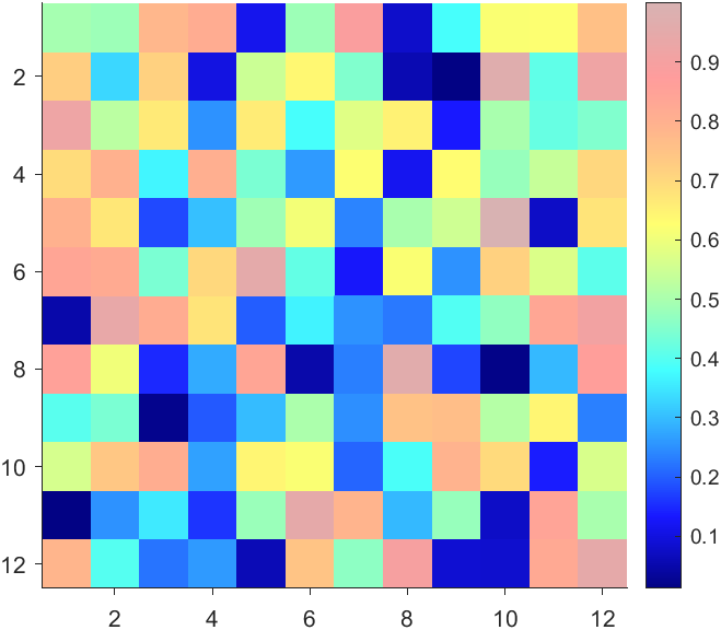
The higher the value, the more transparent it becomes
data = rand(12,12);
AData = rescale(- data, .3, 1);
imagesc(data, 'AlphaData',AData);
colormap(jet);
ax = gca;
ax.DataAspectRatio = [1,1,1];
ax.TickDir = 'out';
ax.Box = 'off';
CBarHdl = colorbar;
pause(1e-16)
CData = CBarHdl.Face.Texture.CData;
ALim = [min(min(AData)), max(max(AData))];
CData(4,:) = uint8(255.*rescale(size(CData, 2):-1:1, ALim(1), ALim(2)));
warning off
CBarHdl.Face.ColorType = 'TrueColorAlpha';
VertexData = CBarHdl.Face.VertexData;
tY = repmat((1:size(CData,2))./size(CData,2), [4,1]);
tY1 = tY(:).'; tY2 = tY - tY(1,1); tY2(3:4,:) = 0; tY2 = tY2(:).';
tM1 = [tY1.*0 + 1; tY1; tY1.*0 + 1];
tM2 = [tY1.*0; tY2; tY1.*0];
CBarHdl.Face.VertexData = repmat(VertexData, [1,size(CData,2)]).*tM1 + tM2;
CBarHdl.Face.ColorData = reshape(repmat(CData, [4,1]), 4, []);
More transparent in the middle
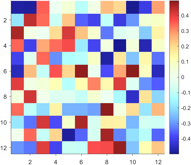
data = rand(12,12) - .5;
AData = rescale(abs(data), .1, .9);
imagesc(data, 'AlphaData',AData);
colormap(jet);
ax = gca;
ax.DataAspectRatio = [1,1,1];
ax.TickDir = 'out';
ax.Box = 'off';
CBarHdl = colorbar;
pause(1e-16)
CData = CBarHdl.Face.Texture.CData;
ALim = [min(min(AData)), max(max(AData))];
CData(4,:) = uint8(255.*rescale(abs((1:size(CData, 2)) - (1 + size(CData, 2))/2), ALim(1), ALim(2)));
warning off
CBarHdl.Face.ColorType = 'TrueColorAlpha';
VertexData = CBarHdl.Face.VertexData;
tY = repmat((1:size(CData,2))./size(CData,2), [4,1]);
tY1 = tY(:).'; tY2 = tY - tY(1,1); tY2(3:4,:) = 0; tY2 = tY2(:).';
tM1 = [tY1.*0 + 1; tY1; tY1.*0 + 1];
tM2 = [tY1.*0; tY2; tY1.*0];
CBarHdl.Face.VertexData = repmat(VertexData, [1,size(CData,2)]).*tM1 + tM2;
CBarHdl.Face.ColorData = reshape(repmat(CData, [4,1]), 4, []);
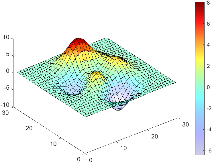
The code will work if the plot have AlphaData property
data = peaks(30);
AData = rescale(data, .2, 1);
surface(data, 'FaceAlpha','flat','AlphaData',AData);
colormap(jet(100));
ax = gca;
ax.DataAspectRatio = [1,1,1];
ax.TickDir = 'out';
ax.Box = 'off';
view(3)
CBarHdl = colorbar;
pause(1e-16)
CData = CBarHdl.Face.Texture.CData;
ALim = [min(min(AData)), max(max(AData))];
CData(4,:) = uint8(255.*rescale(1:size(CData, 2), ALim(1), ALim(2)));
warning off
CBarHdl.Face.ColorType = 'TrueColorAlpha';
VertexData = CBarHdl.Face.VertexData;
tY = repmat((1:size(CData,2))./size(CData,2), [4,1]);
tY1 = tY(:).'; tY2 = tY - tY(1,1); tY2(3:4,:) = 0; tY2 = tY2(:).';
tM1 = [tY1.*0 + 1; tY1; tY1.*0 + 1];
tM2 = [tY1.*0; tY2; tY1.*0];
CBarHdl.Face.VertexData = repmat(VertexData, [1,size(CData,2)]).*tM1 + tM2;
CBarHdl.Face.ColorData = reshape(repmat(CData, [4,1]), 4, []);

I have lon and lat and signal stengths plotting from my roaming GPS Lora module that reports signal strength to Thingspeak at it's location. I got GEOSCATTER plotting location circles.But i want extrapulate?Interp?Heatmap. the stengths between the points. When i use Interp i end up timiming out. How do i modify my code to do this?
Public Channel 214526
Cheers Andy
The study of the dynamics of the discrete Klein - Gordon equation (DKG) with friction is given by the equation :

In the above equation, W describes the potential function: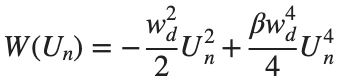
to which every coupled unit  adheres. In Eq. (1), the variable $
 $ is the unknown displacement of the oscillator occupying the n-th position of the lattice, and
  is the discretization parameter. We denote by h the distance between the oscillators of the lattice. The chain (DKG) contains linear damping with a damping coefficient
  , while
 is the coefficient of the nonlinear cubic term.
$ is the unknown displacement of the oscillator occupying the n-th position of the lattice, and For the DKG chain (1), we will consider the problem of initial-boundary values, with initial conditions

and Dirichlet boundary conditions at the boundary points  and
and  , that is,
and , that is,
Therefore, when necessary, we will use the short notation  for the one-dimensional discrete Laplacian
for the one-dimensional discrete Laplacian
Now we want to investigate numerically the dynamics of the system (1)-(2)-(3). Our first aim is to conduct a numerical study of the property of Dynamic Stability of the system, which directly depends on the existence and linear stability of the branches of equilibrium points.
For the discussion of numerical results, it is also important to emphasize the role of the parameter  . By changing the time variable
  , we rewrite Eq. (1) in the form
 . We consider spatially extended initial conditions of the form:
We also assume zero initial velocity:
the following graphs for  and
and 
% Parameters
L = 200; % Length of the system
K = 99; % Number of spatial points
j = 2; % Mode number
omega_d = 1; % Characteristic frequency
beta = 1; % Nonlinearity parameter
delta = 0.05; % Damping coefficient
% Spatial grid
h = L / (K + 1);
n = linspace(-L/2, L/2, K+2); % Spatial points
N = length(n);
omegaDScaled = h * omega_d;
deltaScaled = h * delta;
% Time parameters
dt = 1; % Time step
tmax = 3000; % Maximum time
tspan = 0:dt:tmax; % Time vector
% Values of amplitude 'a' to iterate over
a_values = [2, 1.95, 1.9, 1.85, 1.82]; % Modify this array as needed
% Differential equation solver function
function dYdt = odefun(~, Y, N, h, omegaDScaled, deltaScaled, beta)
U = Y(1:N);
Udot = Y(N+1:end);
Uddot = zeros(size(U));
% Laplacian (discrete second derivative)
for k = 2:N-1
Uddot(k) = (U(k+1) - 2 * U(k) + U(k-1)) ;
end
% System of equations
dUdt = Udot;
dUdotdt = Uddot - deltaScaled * Udot + omegaDScaled^2 * (U - beta * U.^3);
% Pack derivatives
dYdt = [dUdt; dUdotdt];
end
% Create a figure for subplots
figure;
% Initial plot
a_init = 2; % Example initial amplitude for the initial condition plot
U0_init = a_init * sin((j * pi * h * n) / L); % Initial displacement
U0_init(1) = 0; % Boundary condition at n = 0
U0_init(end) = 0; % Boundary condition at n = K+1
subplot(3, 2, 1);
plot(n, U0_init, 'r.-', 'LineWidth', 1.5, 'MarkerSize', 10); % Line and marker plot
xlabel('$x_n$', 'Interpreter', 'latex');
ylabel('$U_n$', 'Interpreter', 'latex');
title('$t=0$', 'Interpreter', 'latex');
set(gca, 'FontSize', 12, 'FontName', 'Times');
xlim([-L/2 L/2]);
ylim([-3 3]);
grid on;
% Loop through each value of 'a' and generate the plot
for i = 1:length(a_values)
a = a_values(i);
% Initial conditions
U0 = a * sin((j * pi * h * n) / L); % Initial displacement
U0(1) = 0; % Boundary condition at n = 0
U0(end) = 0; % Boundary condition at n = K+1
Udot0 = zeros(size(U0)); % Initial velocity
% Pack initial conditions
Y0 = [U0, Udot0];
% Solve ODE
opts = odeset('RelTol', 1e-5, 'AbsTol', 1e-6);
[t, Y] = ode45(@(t, Y) odefun(t, Y, N, h, omegaDScaled, deltaScaled, beta), tspan, Y0, opts);
% Extract solutions
U = Y(:, 1:N);
Udot = Y(:, N+1:end);
% Plot final displacement profile
subplot(3, 2, i+1);
plot(n, U(end,:), 'b.-', 'LineWidth', 1.5, 'MarkerSize', 10); % Line and marker plot
xlabel('$x_n$', 'Interpreter', 'latex');
ylabel('$U_n$', 'Interpreter', 'latex');
title(['$t=3000$, $a=', num2str(a), '$'], 'Interpreter', 'latex');
set(gca, 'FontSize', 12, 'FontName', 'Times');
xlim([-L/2 L/2]);
ylim([-2 2]);
grid on;
end
% Adjust layout
set(gcf, 'Position', [100, 100, 1200, 900]); % Adjust figure size as needed
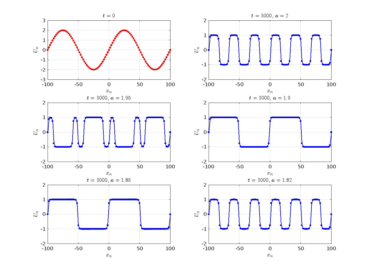
Dynamics for the initial condition ,  , for
, for  , for different amplitude values. By reducing the amplitude values, we observe the convergence to equilibrium points of different branches from
  and the appearance of values
  for which the solution converges to a non-linear equilibrium point
  Parameters:
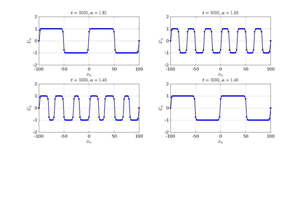
Detection of a stability threshold  : For
: For  , the initial condition ,
  , converges to a non-linear equilibrium point
 .
.
Characteristics for  , with corresponding norm
  where the dynamics appear in the first image of the third row, we observe convergence to a non-linear equilibrium point of branch
  This has the same norm and the same energy as the previous case but the final state has a completely different profile. This result suggests secondary bifurcations have occurred in branch
where the dynamics appear in the first image of the third row, we observe convergence to a non-linear equilibrium point of branch By further reducing the amplitude, distinct values of  are discerned: 1.9, 1.85, 1.81 for which the initial condition
  with norms
  respectively, converges to a non-linear equilibrium point of branch
  This equilibrium point has norm
  and energy
  . The behavior of this equilibrium is illustrated in the third row and in the first image of the third row of Figure 1, and also in the first image of the third row of Figure 2. For all the values between the aforementioned a, the initial condition
  converges to geometrically different non-linear states of branch
  as shown in the second image of the first row and the first image of the second row of Figure 2, for amplitudes
  and
and  respectively.
respectively, converges to a non-linear equilibrium point of branch and energy Refference: