Results for
We are nearly at the anniversary of The Great Outage, May 19 2025 to May 27 2025. At the time, many Mathworks services were down due to a ransomware attack.
Some service was restored by May 21 2025 but it went down again after that.
I see some indication that some features such as @doc took even longer to restore than May 27th.
The outage came as MATLAB Answers usage was already declining a fair bit due to widespread AI use, and unfortunately some of the existing traffic just never came back.
We’re excited to share that Cleve Moler, creator of MATLAB, has been elected to the U.S. National Academy of Sciences—one of the highest honors in science.
This recognition celebrates Cleve’s groundbreaking contributions to numerical computing and his lasting impact on researchers, educators, and engineers around the world. From advancing numerical linear algebra to making powerful computation more accessible through MATLAB, his work has shaped how science and engineering are done today.
Please join us in congratulating Cleve on this well‑deserved honor!
🔗 Learn more about the 2026 NAS election
Hey AI, add computation to my modern physics course. Thanks.
Duncan Carlsmith
Department of Physics, University of Wisconsin-Madison
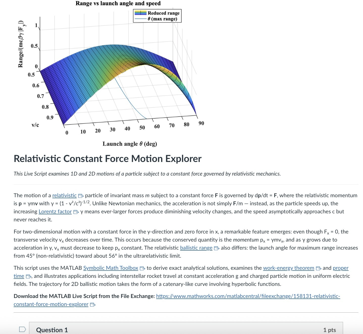
An AI-generated CANVAS quiz header based on a Live Script on relativistic motion.
Introduction
Agentic AI is disrupting higher education. An agentic AI can act on the web rather than relying solely on its training. It can research a topic and produce a credible research paper to specification with validated references. It can create, answer, or assess student work on physics questions from elementary mechanics to graduate-level quantum field theory or quantum computing. It can comprehend, generate, run, and debug a MATLAB Live Script zip package, an HTML5 interactive web application, a JavaScript-enabled website, an ADA-compliant CANVAS site with math and images, or a mobile phone app. A student can authenticate in a learning management system like CANVAS and issue a simple prompt to an agentic AI — “Complete all of my assignments in all of my courses. Thanks.” — and an instructor can, on the other side, with AI assistance and a simple prompt, assess all such submissions, even messy hand-written work. I have demonstrated these capabilities and others.
Here, I’d like to share an experiment leveraging AI to inject computation with MATLAB into a course in modern physics. This may interest the academic readers of this blog and the curious. My prior post Giving All Your Claudes the Keys to Everything introduced my personal agentic AI context.
Live Script goals
Some years back now, I started developing and introducing Live Scripts in a two-semester introductory physics course to immerse students in computation and science without sacrificing the rigor and breadth of the class. These students have essentially no background in computing and are exploring STEM majors — physics, astronomy, and engineering principally. A self-documenting Live Script allows a student to explore even a relatively advanced physics topic and data analysis trick like Fourier analysis or autocorrelation, using data like a mobile phone voice memo or a digital oscilloscope output race that they collect themselves, and then apply the same techniques to analyze big science open data from for example as gravitational wave observatory, both without being mired down in mathematics or code writing. As the course evolves, computational challenges connected to the laboratory component introduce much of the gamut of MATLAB functionality. The goal is to show why and how modeling and assessment using computation are essential in science, and to empower students with practical skills and a sense of what is possible. The traditional lecture/demonstration/homework/discussion format was largely untouched. This course sequence was a five-credit automatic honors course, so extra work was expected. Coding as a tool rather than a chore or vocation is all the more relevant in the AI age.
Assessment strategy
To flexibly direct and assess student work, each Live Script contains a variety of ‘Try this’ suggestions which require the user to adjust a parameter or two and observe the consequences. The student must study the physics described in the background information section, and the code enough to understand how the code logic works, using the supplied comments and URLs to documentation. Tackling a ‘Try this ‘ suggestion does not require any coding, just changing a parameter value, perhaps with a slider. Additionally, the Live Script contains ‘Challenges’ to extend the code in some simple or possibly advanced way. The Live Script can thus serve different customers, and an instructor can further tailor the script and embedded suggestions and challenges as they choose. The possibilities offered are only exemplary.
An associated CANVAS quiz contains a few multiple-choice questions related to the ‘Try this’ suggestions, which are auto-graded. Additional questions require the student to upload a product, like an appropriately labeled plot comparing data to a model fit, together with a written explanation. These are readily graded electronically using CANVAS SpeedGrader, with or without an e-rubric. The emphasis is on results and analysis, not on coding facility or style. By design, the burden on the instructor is minimal.
AI-generated computational thread
In teaching a 3-credit third-semester survey of modern physics (relativity, quantum mechanics, atomic, molecular, solid state, nuclear, particle, and astro physics) without a lab and again for students with little or no prior exposure to computation, I needed first to develop more advanced, relevant Live Scripts. This course offers three lecture hours per week, rife with live demonstrations of cathode ray tubes, electron diffraction, Geiger counters and sources, thermal radiation, the photoelectric effect, gas discharge tubes observed with diffraction glasses, lasers, and magnetic levitation with diamagnetic and high temperature superconductors, and so on. An additional mandatory hour per week is dedicated to small group active learning in sectional meetings. A contemporary e-text and integrated WebAssign homework system are linked via LTI to CANVAS. These components address learning goals I am loath to sacrifice. I ultimately decided to make the new computational thread an attractive extra-credit option (in parallel with a research paper option) and implemented it with AI assistance mid-stream this semester in a way that could be emulated.
The agent was Claude Desktop running with MCP servers: the Playwright browser-automation server (for CANVAS interaction via authenticated browser session), MATLAB MCP server to run MATLAB, and a filesystem server (for reading local Live Script packages and writing artifacts back to disk). I asked Claude to survey my modern physics syllabus on CANVAS and my 150+ Live Scripts on the MATLAB File Exchange (FEX), and to identify those relevant to a 3rd-semester course in relativity, quantum mechanics, atomic, molecular, solid state, nuclear, particle, and astro physics, with my Introduction to MATLAB script included as a foundations option. Claude returned an initial list of 38 candidate scripts. I removed two that were not a good fit and approved 14, including chaos in relativistic mechanics, relativistic motion in a Coulomb field, numerical solutions to the Schrödinger equation in 1D/2D/3D via the PDE Toolbox, gravitational-wave data analysis, exoplanet transit detection, and clustering in Gaia mission stellar data, among others.
For each approved script, Claude downloaded the FEX zip via MATLAB websave and unzip, converted the .mlx to readable .m text via matlab.internal.liveeditor.openAndConvert, ran the key numerical sections in MATLAB to obtain concrete answer values, and then used a single Playwright browser_evaluate call — authenticated by the CSRF token from the active CANVAS browser cookie — to POST a new quiz plus all of its questions to the CANVAS REST API in one round trip. (The MATLAB webwrite path with a CANVAS_API_TOKEN environment variable consistently returned 401 in our testing; the browser-session approach worked reliably for all 14 quizzes.)
Each quiz is structured identically: a description block with the FEX thumbnail image, a two- to three-paragraph physics introduction essentially copied from the FEX page or script itself with Wikipedia links to technical terms, a download link, and an “Open in MATLAB Online” link; followed by 4 multiple-choice questions worth 1 pt each (covering a fundamental physics fact, a physical mechanism, an experimental or computational technique, and a data-analysis concept), and 3 essay questions worth 3 pts each (a basic execution + screenshot, a quantitative comparison, and a bonus “Try this” modification). The essay type was deliberate: a CANVAS file_upload question accepts only a file, while an essay question gives the student a Rich Content Editor in which they can paste a screenshot directly from the clipboard and type their analysis in the same field. SpeedGrader then shows everything together. We also added an optional 0-credit student feedback question that we crafted jointly. Total: 13 points per quiz.
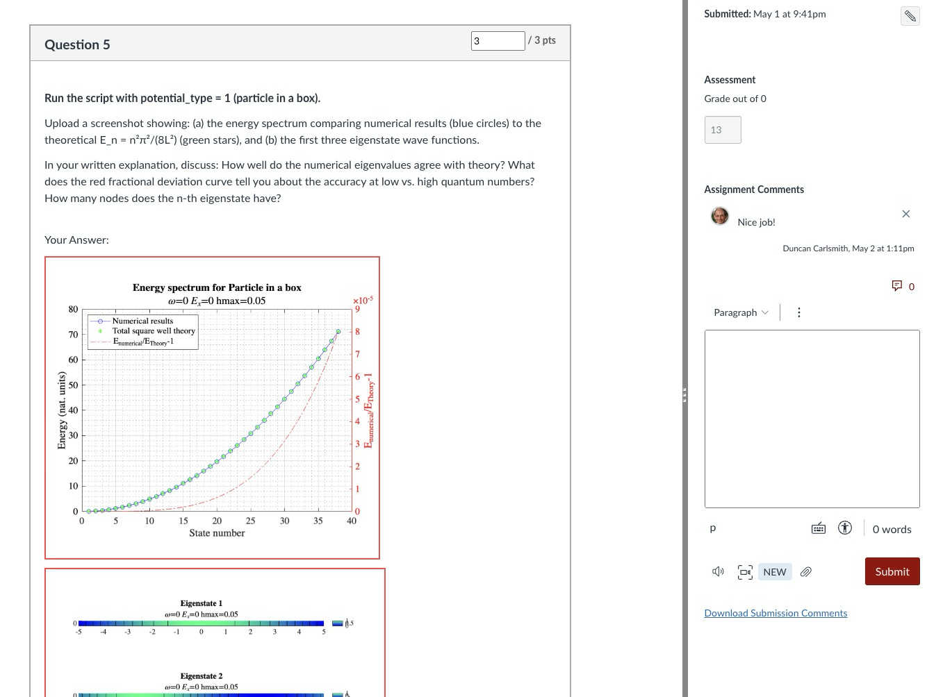
Speed Grader view of a Rich Content Editor question with uploaded results
The full set of 14 quizzes was created in a single working session. I reviewed and accepted the results essentially without revision — a few quiz descriptions needed a follow-up PUT to fix image sizing or to add the MATLAB Online link, but no question content required rewriting. Across the session, the procedure crystallized into a reusable SKILL.md that documents the FEX-to-CANVAS recipe end to end (download with MATLAB, design questions in the four-category MC pattern, batch quiz + question creation, verification checklist).
An AI touch on grading made the assignment fit the course without inflating its weight: a 5% group weight on the Computation category, with a drop-lowest-eleven-of-fourteen rule that keeps each student’s top three quizzes. Each quiz is 13 points, so the maximum contribution is (39/39) × 5% = 5.00% extra credit, and any student can attempt as few or as many as they wish without exceeding that cap. The CANVAS configuration is non-trivial in a few ways and includes one gotcha worth knowing about; details are in Appendix A.
Outcomes
I received about 75 submissions, with 30 of the 75 students participating, and many others opting for the research paper. Feedback was generally positive. Only a few students ran into difficulty: one suffered a European Space Agency network outage while accessing Gaia data, and another had trouble with a screen-capture process unrelated to MATLAB. Students reported workloads in an appropriate 1–3 hour range per assignment. Only about 20% of submitters elected to submit the (quite lengthy) Introduction to MATLAB assignment for credit; some likely encountered MATLAB already in the math department or engineering school, where it is used extensively, and others may have reviewed the assignment but elected not to submit because the upload questions concerned image processing (compression and decompression, blurring and deblurring) rather than course-relevant topics. Several students volunteered that these exercises were more informative and fun than their canonical problem-solving exercises.
Lessons
A few patterns from this experiment seem worth carrying forward. First, the ‘Try this’ design pattern that I had already adopted turns out to be unusually well suited to AI-assisted assessment: each suggestion converts almost mechanically into a three-part question (run, capture, analyze) with a defensible rubric; Hence one working session yielded a full term’s worth of quizzes. Second, the agentic build is a short, explicit recipe — read the script, run the calculations, design the questions, post via the CANVAS API in one batched call — that other instructors can replicate and which is now captured for me in a SKILL.md. Third, the Canvas grading mechanics (drop-lowest, keep-best-three, group weight cap) let extra-credit work scale gracefully: students self-select breadth versus depth, and the instructor’s exposure to grading volume is bounded.
Conclusions
More broadly, I expect education to become more efficient and engaging in this AI age, with much of the routine instructional and learning burden relegated to AI. Frontier AIs can affordably tutor undergraduate students and even PhDs at their level and challenge them in new ways and at scale. Students and instructors both must develop and adjust to new learning strategies and expectations. Documented exploration enabled by interactive, code-aware artifacts like Live Scripts and Jupyter notebooks, created by a student or researcher collaboratively with AIs and other compatriots, may play an ever more important role in this environment.
My SKILL.md is 665 lines and specific to my setup, so not shared here. You might be asking an AI to install Chromium and Playwright or Puppeteer and do all the work in its container. You might be electing a different assignment structure, accessing your own Live Scripts or Python equivalent located at GitHub or someplace other than the MATLAB FEX. This article documents most of what is in my skill file and would be useful background information. You will want to develop and test your own process if emulating the idea here.
Acknowledgements and disclosure
The products described here and this essay were prepared with the assistance of Claude.ai. The author declares he has no financial interest in Anthropic or MathWorks.
Appendix A: CANVAS gradebook configuration
The intent was simple to state: a student who completes three or more MATLAB quizzes at full marks should receive the full 5% extra-credit boost on their course total; a student who completes one quiz at full marks should receive one-third of that boost; a student who attempts none should receive nothing. Implementing this in CANVAS took three coordinated pieces, each of which is straightforward in isolation but has at least one non-obvious failure mode.
A.1 Group structure and drop rule. The 14 quizzes live in a single assignment group named “Computation,” weighted at 5% of the course grade. The group has one rule: drop the lowest 11 scores. With 14 assignments and 11 dropped, CANVAS keeps each student’s top three. Each quiz is worth 13 points (4 multiple-choice at 1 pt + 2 essay at 3 pts + 1 bonus essay at 3 pts), so the maximum sum across the kept three is 39, and the maximum group percentage is 39/39 = 100%, contributing 0.05 × 100% = 5.00% to the course total. The group weight thus acts as a hard ceiling: no matter how many quizzes a student attempts, their boost cannot exceed 5%.
A.2 Treating ungraded as zero, selectively. Out of the box, CANVAS treats ungraded assignments as ignored rather than as zero. This is usually the right default — a student who has not yet attempted an assignment is not penalized for it — but it interacts badly with the design intent here. If a student attempted exactly one MATLAB quiz and scored 13/13, CANVAS would show their Computation group total as 13/13 = 100%, awarding the full 5% boost for a single quiz. To get the intended scaling (one quiz at 13/13 should yield 13/39 = 33.33%, contributing 1.67% rather than 5%), the unattempted quizzes must count as zero in the group calculation.
The simplest way to enforce that globally is the gradebook setting Treat Ungraded as 0, but this applies course-wide and was undesirable in my case because of an exam-administration mixup in which different students had taken different versions of Exam 1; only the version each student took should count toward their exam grade, and a global “treat ungraded as 0” would have penalized students for the version they had not been assigned. The per-assignment alternative is to use the gradebook column menu (the three-dot menu on each assignment column) and choose Set Default Grade, entering 0 with the “Overwrite already-entered grades” box left unchecked. This converts every dash in that column to a 0 while leaving real scores untouched, and only affects the assignment whose menu was used. Applied to each of the 14 MATLAB quizzes, this gives the desired “ungraded as zero” behavior in the Computation group without affecting Exam 1 or any other category. After the fix, the worked examples behave as expected..
A.3 The points_possible gotcha. When a CANVAS Classic Quiz is created via the REST API and the quiz’s questions are POSTed in subsequent calls (or even, as in our case, in the same browser_evaluate call but as separate POST requests), the assignment row that mirrors the quiz in the gradebook can retain points_possible = 0 even though the questions internally sum to 13. The quiz preview displays the question points correctly, the quiz statistics show the correct totals, but the gradebook column header reads “Out of 0” and the group percentage calculation collapses to nonsense. Symptomatically, a student with one real score appeared at 30.77% in the Computation column when they should have been at 33.33% — the column was contributing 4/13 instead of 4/39 because 13 of the 14 columns were silently weightless.
The cure is to force CANVAS to recompute the assignment row’s points_possible from the question sum. The simplest way is per-quiz from the UI: open the quiz, click Edit, scroll to the bottom of the editor without changing anything, and click Save (not “Save & Publish” if the quiz is already published). The act of saving the quiz triggers the recompute. The same effect is available via the API by issuing PUT /api/v1/courses/{course_id}/assignments/{assignment_id} with body {"assignment": {"points_possible": 13}} on each affected assignment, which is faster for batch use.
The lesson for anyone scripting CANVAS quiz creation: after batch-creating quizzes and questions via the API, always verify the gradebook column header reads “Out of N” with N matching the question sum, and apply one of the two cures above before students start submitting. The skill file used in this project now flags this check explicitly.
Mitigating chat failures in AI code development
Duncan Carlsmith
Department of Physics, University of Wisconsin-Madison
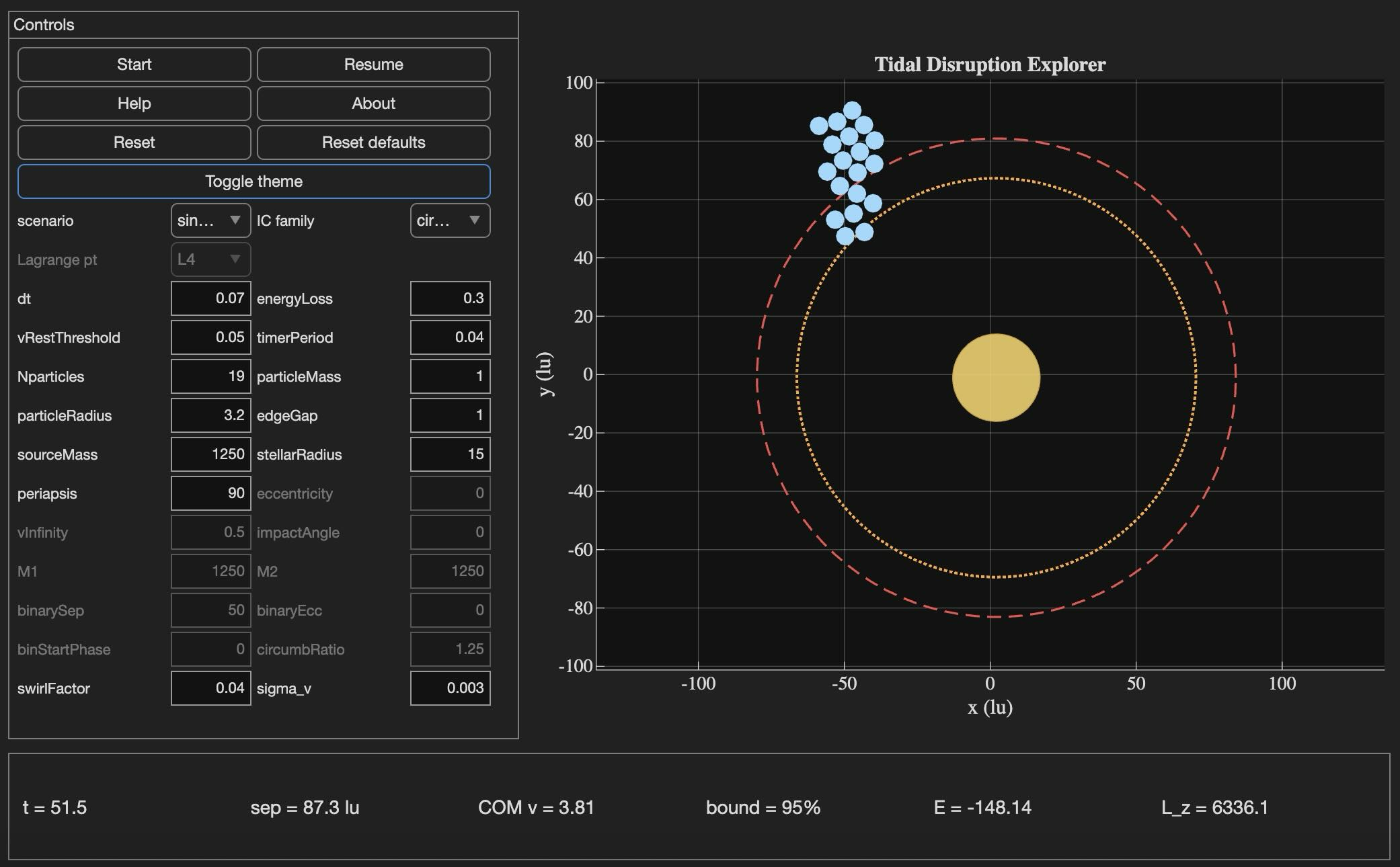
Tidal Disruption Explorer (MATLAB File Exchange 183760). The process of porting this Live Script ito HTML is described in this post.
Introduction
An agentic AI session ended for me this week with the message: "Claude is unable to respond to this request, which appears to violate our Usage Policy. Please start a new chat." Gulp. The substance of the conversation was completely benign — porting my MATLAB Live Script Tidal Disruption Explorer that simulates a self-gravitating cluster of particles being shredded by tidal forces near a massive object, like Comet Shoemaker-Levy 9 was shredded by Jupiter in 1992. The next chat picked up the work and finished it in seven turns.
Why nothing was lost is the subject of this post. The new product is the HTML5 port of Tidal Disruption Explorer and deployed at duncancarlsmith.github.io/TidalDisruptionExplorer-HTML5. But the more transferable product may be practices that can help make AI-assisted code development resilient to chat failures, connection drops, sandbox losses, and content-policy false positives. Two prior posts set my context: Live Script deployed as a 3D web application with AI introduced the workflow, and Giving All Your Claudes the Keys to Everything introduced the ngrok command server that makes the Mac controllable from any AI client. This post is about how to use such tools without losing your work when the chat dies.
Failure modes worth designing for
Long agentic sessions can fail in many ways, and most are out of the user's control. The bash_tool connection in the cloud container can go unresponsive mid-task. A stray Python process can mask a real command server on the same port. A lost development sandbox can vaporize generated artifacts — in an earlier turn of this same project, an entire test-harness directory disappeared with the sandbox and had to be reconstructed from the conversation log. Persistent context is not in fact persistent. Skills are forgotten. The user closes the laptop, the WiFi blinks off, or the chat hits a length limit. This project used Claude, but the problems are not AI-specific in my experience with 5-6 leading vendors. Without preparation, each of these is a real setback.
Best practices to consider
1. Externalize project state in a committed PROGRESS journal
A single file, committed in a repo, names every milestone, the test-pass count for each, the current state in prose, and an explicit "Recovery instructions for a fresh session" section that lists the source files, the test harness names, and the toolchain assumptions. When the previous chat failed, the next one resumed from this file alone, without needing the failed conversation. When the dev sandbox loss took out 10 test harnesses, they were rebuilt from the conversation log because the journal had recorded exactly what each harness checked and the expected pass count for each. These harnesses are also stored locally when complete and successful.
2. Two external locations:
The container contents are fragile even without a chat failure due to context compaction and hidden file management. I chose a local working directory as the editable source of truth. A GitHub repository was the final product and might have been used rather than my local storage - that choice was a matter of familiarity and trust. Each change was written locally first via the command server, verified on disk by reading it back, then committed and pushed to GitHub.
3. Run browser tests in the AI's container, not on the user's machine
For this project, the final product was a web app. In prior work, I used a local Chromium to view and test the product. It turns out that Claude's container ships with Node and Playwright preinstalled, and Chromium may be available from the Puppeteer install. Browser regression tests for the HTML5 application were run there entirely, and I only viewed staged intermediate products. Containing the development is not possible when building a MATLAB product without the added burden of using MATLAB in the cloud. The idea was to do as much as possible without overhead in the AI container.
4. Multistep plan with explicit approval gates
Decompose the work into milestones with sub-milestones. Each has a test harness with a documented expected pass count and a concrete deliverable. Don't merge "running a test" with "uploading the result" with "committing the change" — these separate decisions each has its own approval and verification. If the chat dies between any two of them or something else goes awry, the user can stop without leaving anything dangling. This project: 8 milestones, 27 sub-milestones, 260 documented sub-checks.
5. Versioned backups before any destructive write
Every PROGRESS edit got a timestamped pre-edit copy first in the local project repo, one per milestone.
Result
Recovery from the failed chat only cost me one turn. Six more turns to finish the project. The final result: 260 of 260 sub-checks pass across all milestones, live deployment verified. Many hairs pulled (the violation of usage policy issue was not the only one encountered!), but no utter despair experienced!
Links
Live HTML5 application: https://duncancarlsmith.github.io/TidalDisruptionExplorer-HTML5/
MATLAB Live Script (File Exchange 183760): https://www.mathworks.com/matlabcentral/fileexchange/183760-tidal-disruption-explorer
Source repository (GitHub): https://github.com/DuncanCarlsmith/TidalDisruptionExplorer-HTML5
Starting in R2026a you can export MATLAB figures to an HTML file that preserves axes interactions.
Click on the figure below to open the interactive MATLAB figure and pan or zoom into the axes. This demo also uses a new linkaxes feature available in R2026a.
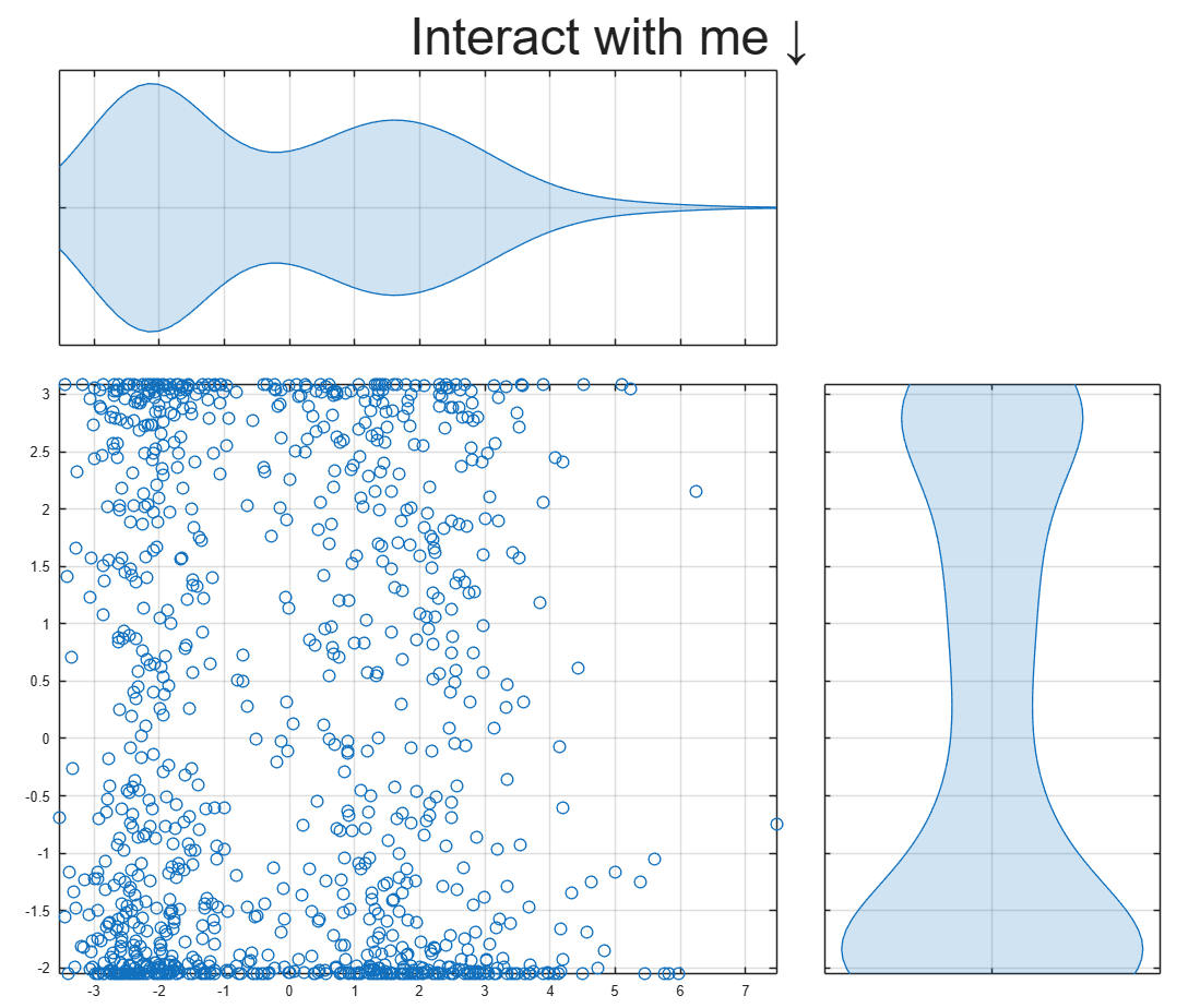
To learn about more Graphics and App Building features in R2026a, check out today's blog article:
I submitted a Matlab support case but posting this publicly to hopefully save people some trouble and see if anyone has ideas.
After upgrading my workstation from Ubuntu 25.10 to Ubuntu 26.04 LTS, MATLAB GUI consistently prints this terminal error on shutdown:
free(): chunks in smallbin corrupted
MATLAB appears to run normally, but closing the GUI takes a long time and sometimes produces crash dumps. The terminal error occurs every time I close the GUI, but crash dumps are intermittent. I attached one R2026a crash dump. I had zero issues on Ubuntu 25.10.
Affected versions:
- MATLAB R2026a
- MATLAB R2025b
- I suspect any 'new desktop' version
System:
- Ubuntu 26.04 LTS
- AMD EPYC 7443P
- NVIDIA RTX 3090
- Ubuntu 26.04 default NVIDIA driver: nvidia-driver-595-open, 595.58.03
- NVIDIA module path: /lib/modules/7.0.0-14-generic/kernel/nvidia-595-open/nvidia.ko
- glibc 2.43
Important note: the error first occurred with a clean MathWorks MATLAB installation before installing the Ubuntu/Debian `matlab-support` package. I later tested after installing `matlab-support`, which I understand modifies/renames some MATLAB-bundled libraries so MATLAB uses selected system libraries instead. The same shutdown error occurs both before and after applying `matlab-support`. This suggests the issue is not caused solely by the Debian/Ubuntu `matlab-support` integration or solely by one of the libraries it substitutes.
The attached crash dump shows abort/free() heap corruption detected in libc, but the higher-level stack includes MATLAB libraries such as:
- libmwcppmicroservices.so
- libmwmodule_descriptor_implementation.so
- libmwmatlab_main_lib.so
- libmwfoundation_threadpool.so
The issue appears GUI-specific. Using these startup flags shut down cleanly:
- matlab -batch
- matlab -nodesktop
- matlab -nodisplay
The shutdown error still occurs with these startup flags:
- normal GUI launch
- -nosplash
- -nojvm
- -softwareopengl
- -cefdisablegpu
The issue also persists after:
- renaming/resetting ~/.matlab/R2026a and ~/.MathWorks/R2026a
- launching with a clean environment without LD_LIBRARY_PATH, LD_PRELOAD, MATLAB_JAVA, JAVA_HOME, JRE_HOME, etc.
- testing a new Ubuntu user account
- testing Ubuntu/GNOME, GNOME, and Xfce X11 sessions
- testing NO_AT_BRIDGE=1 and GTK_USE_PORTAL=0
- temporarily moving ~/.MathWorks/ServiceHost
- testing GLIBC_TUNABLES=glibc.malloc.tcache_count=0
- trying to capture a system coredump with ulimit -c unlimited / coredumpctl; no system coredump was produced
Because R2025b and R2026a are both affected, terminal-only modes exit cleanly, the problem occurs across GNOME/Wayland and Xfce/X11, and the error occurred on a clean MATLAB install before any `matlab-support` modifications, this appears related to MATLAB GUI shutdown on Ubuntu 26.04 / glibc 2.43 rather than a corrupted MATLAB preference folder, a single desktop session, or the Ubuntu `matlab-support` package.
Example crash dump:
Hi everyone
My blog post about the latest MATLAB release was published yesterday MATLAB R2026a has been released – What’s new? » The MATLAB Blog - MATLAB & Simulink
There are a lot of new features and performance enhancements and from conversations I've had across several social media platforms., it seems that the new metafunction functionality is emerging as a user favourite. What are you most excited to see?
Cheers,
Mike
Hi,
I am trying to use an esp32 board with quectal ec200u LTE Modem to send sensor data to thingspeak. The board can process the sensor data however I am unable to send the data to thingspeak. I have used the same process earlier too however with a different modem from Simcom.
Can someone help me with specific commands for achieving this? I can share the code which i am trying to use.
Regards
Aditya
Good morning everyone. I’m having a problem with ThingSpeak. I’m sending data from an ESP LoRa with the RTC set to the Brasília time zone (GMT-3).
Previously, when I exported the data to CSV, it used the ThingSpeak time, which appeared 3 hours ahead. Now that I’m sending the timestamp from the ESP, the graphs are showing the data 3 hours behind. Is there a way to align the graph times while keeping the Brazilian time zone?
I have been a loyal MATLAB user for 25 years, starting from my university days. While many of my peers migrated to Python, I stayed for the stability, compatibility, and clean environment. However, I am finding the 2025 version exceptionally laggy. Despite running it on an $10k high-end machine, simple tasks like viewing variables and plotting take up to 60 seconds - actions that were near instantaneous in the 2020 version. I want to stay continue with MATLAB, but this performance gap is a major hurdle and irritation. I hope these optimization issues can be addressed quickly.
Short version: MathWorks have released the MATLAB Agentic Toolkit which will significantly improve the life of anyone who is using MATLAB and Simulink with agentic AI systems such as Claude Code or OpenAI Codex. Go and get it from here: https://github.com/matlab/matlab-agentic-toolkit
Long version: On The MATLAB Blog Introducing the MATLAB Agentic Toolkit » The MATLAB Blog - MATLAB & Simulink
MATLAB EXPO India | 7 May | Bengaluru
Get inspired by the latest trends and real-world customer success stories transforming industries. Learn from trusted experts across 4 tracks.
- AI & Autonomous Systems
- Electrification
- Systems & Software Engineering
- Radar, Wireless & HDL
Register at bit.ly/matlabexpocommunity

Do we know if MATLAB is being used on the Artemis II (moon mission) spacecraft itself? Like is the crew running MATLAB programs? I imagine it was probably at least used in development of some of the components of the spacecraft, rockets, or launch building. Or is it used for any of the image analysis of the images collected by the spacecraft?
MATLAB interprets the first block of uninterupted comments in a function file as documentation. Consider a simple example.
% myfunc This is my function
%
% See also sin
function z = myfunc(x, y)
z = x + y;
end
Those comments are printed in the command window with "help myfunc" and displayed in a separate window with "doc myfunc". A lot of useful things happen behind the scenes as well.
- Hyperlinks are automatically added for valid file names after "See also".
- When dealing with classes, the doc command automatically appends the comment block with a lists of properties and methods.
All this is very handy and as been around for quite some time. However, the doc browser isn't great (forward/back feature was removed several versons ago), the text formatting isn't great, and there is no way to display math.
Although pretty text/math can be displayed in a live document, the traditional *.mlx file format does not always play nice with Git and I have avoided them. However, live documents can now (since 2025a?) be saved in a pure text format, so I began to wonder if all functions should be written in this style. Turns out that all you have to do is append these lines:
%[appendix]{"version":"1.0"}
%---
to the end of any function file to make it a live function. Doing so changes how MATLAB manages that first comment block. The help command seems to be unaffacted, although [text] may appear at the start of each comment line (depending on if the file was create as a live function or subsequently converted). The doc command behaves very different: instead of bringing up the traditional window for custom documentation, the comment block looks like it gets published to HTML and looks more similar to standard MATLAB help. This is a win in some ways, but the "See also" capabilitity is lost.
Curiously, the same text can be appended to the end of a class definition file with some affect. It does not change how the file shows up in the editor, but as in live functions, comments are published when using the doc command. So we are partway to something like a "live class", but not quite.
Should one stick with traditional *.m files or make everything live? Neither does a great job for functions/classes in a namespace--references must explicitly know absolute location in traditional functions, and there is no "See also" concept in a live function. Do we need a command, like cdoc (custom documentation), that pulls out the comment block, publishing formatted text to HTML while simultaneously resolving "See also" references as hyperlinks? If so, it would be great if there were other special commands like "See examples" that would automatically copy and then open an example script for the end user.
Hi all,
I'm a UX researcher here at MathWorks working on the MathWorks Central Community. We're testing a new feature to make it easier to ask a question, and we'd love to hear from community members like you.
Sessions will be next week. They are remote, up to 2 hours (often shorter), and participants receive a $100 stipend. If you're interested, you can click here to schedule.
Thanks in advance! Your feedback directly shapes what gets built.
--David, MathWorks UX Research
Digital Twin Development of PEARL Autonomous Surface System Thermal Management
The top session of the countdown showcases how the PEARL engineering team used a digital twin to solve real‑world thermal challenges in a solar‑powered autonomous marine platform operating in extreme environments. After thermal shutdown events in the field, the team built a model that predicts temperatures at multiple locations with ~1% accuracy, while balancing accuracy with model complexity.
Beyond the technology, this keynote delivers practical lessons for predictive modeling and digital twins that apply well beyond marine systems.
We hope you’ve enjoyed the Top 10 countdown series—and a big thank‑you to Olivier de Weck at Massachusetts Institute of Technology, for delivering such a compelling and insightful keynote.
🎥 If you missed it live, be sure to watch the recording to see why it earned the #1 spot at MATLAB EXPO 2026.

MATLAB EXPO India is Back!
This in-person events brings together engineers, scientists, and researchers to explore the latest trends in engineering and science, and discover new MATLAB and Simulink capabilities to apply to your work.
May 7, 2026 l Bengaluru
Register at bit.ly/matlabexpocommunity
Missed the Cody World Cup Watch Party on March 27—or want to relive the glory?
What you’ll see in the video:
🔥 Top MATLAB users in action
Watch expert solvers think, debug, strategize—and occasionally panic.
Which functions do they reach for? How do they break down the problem?
BEHOLD the power moves… and the 3D arrays.
🏆 Three teams. Six champions. One viciously clever problem.
There may have been NaN traps.
There may have been nested for‑loops.
There may have been… emotions.
🎙️ Professional‑grade commentary by:
@Matt Tearle – Architect of Diabolical Challenges
Their line‑by‑line play‑by‑play turns MATLAB into a true spectator sport.
Finally, tell us what you want to see next—head‑to‑head contests? Team battles? Drop your ideas in the comments. All suggestions welcome!
Hello Community,
Registration is now open for the MathWorks Automotive Conference 2026 North America. Join industry leaders and MathWorks experts to learn about the latest trends in:
- Software-defined vehicles
- Generative AI
- Virtual vehicles
- AI and machine learning
Event details
- Date: April 28, 2026
- Location: Saint John’s Resort, Plymouth, MI
This conference is a great opportunity to connect with MathWorks and industry peers—and to explore what’s next in automotive engineering. We encourage you to register today.
We hope to see you there.
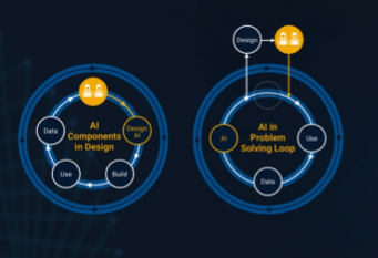
It’s no surprise this keynote landed at #2. MaryAnn Freeman, Senior Director of Engineering, AI, and Data Science explores how AI, especially generative AI, is transforming the way engineers design, build, and innovate. From accelerating the design loop with faster, data‑driven solutions, to blending human creativity with AI insights, to evolving engineering tools that turn ideas into build‑ready systems. This keynote shows how embedded intelligence helps engineers push past traditional limits and bridge imagination with real‑world impact.
If you’re curious about how AI is reshaping engineering workflows today (and what that means for the future of design), this is a must‑watch.
👉 Watch the keynote recording and see why it was one of the most popular sessions of MATLAB EXPO Online 2025.