Results for
As of an hour ago my Visualisation stopped working, suddenly returning an empty matrix for 'old' (2019) data retrieved. It has been working fine all day and historically. New data being uploaded today is being retrieved fine. My code hasn't changed.
Downloading and checking, all data prior to 29-Nov-2023 has gone.
Has something changed server side?
Have you ever used Live Tasks in MATLAB? MathWorks development team would like to get some feedback on your experience – what did you like and not like. Especially, if you know about it but don’t use it frequently, we would like to understand why?
Please tell us what you think by submitting your response to this form https://forms.office.com/r/ui1EGqAFDx
how accurate are the answers of the AI Playground regarding information that are not specifiyed in the documentation?
A key aspect to masting MATLAB Graphics is getting a hang of the MATLAB Graphics Object Hierarchy which is essentially the structure of MATLAB figures that is used in the rendering pipeline. The base object is the Graphics Root (see groot) which contains the Figure. The Figure contains Axes or other containers such as a Tiled Chart Layout (see tiledlayout). Then these Axes can contain graphics primatives (the objects that contain data and get rendered) such as Lines or Patches.
Every graphics object has two important properties, the "Parent" and "Children" properties which can be used to access other objects in the tree. This can be very useful when trying to customize a pre-built chart (such as adding grid lines to both axes in an eye diagram chart) or when trying to access the axes of a non-current figure via a primative (so "gca" doesn't help out).
One last Tip and Trick with this is that you can declare graphics primatives without putting them on or creating an Axes by setting the first input argument to "gobjects(0)" which is an empty array of placeholder graphics objects. Then, when you have an Axes to plot the primitive on and are ready to render it, you can set the "Parent" of the object to your new Axes.
For Example:
l = line(gobjects(0), 1:10, 1:10);
...
...
...
l.Parent = gca;
Practicing navigating and exploring this tree will help propel your understanding of plotting in MATLAB.
One of my colleauges, Michio, recently posted an implementation of Pong Wars in MATLAB
- Here's the code on GitHub.https://lnkd.in/gZG-AsFX
- If you want to open with MATLAB Online, click here https://lnkd.in/gahrTMW5
- He saw this first here: https://lnkd.in/gu_Z-Pks
Making me wonder about variations. What might the resulting patterns look with differing numbers of balls? Different physics etc?
We're thrilled to announce the roll-out of some new features that are going to supercharge your Playground experience! Here's what's new:
Copy/Download code from the script area
You can now effortlessly Copy/Download code from the script area with just a single click. Copy code or Download your script directly as .m files and keep your work organized and portable.We hope this will allow you to effortlessly transfer your work from Playground to MATLAB Desktop/Online.
Run Code directly from the Chat panel
Execute code snippets from the chat section with a single click. This new affordance means saving a step since you no longer have to insert code and then hit run from the toolstrip to execute instead just hit run in the chat panel to see the output immediately in the script area
Enhanced visual Experience
Customize your Playground workspace by expanding or collapsing the chat and script sections. Focus on what matters most to you, whether it's AI chat or working on your script.
We hope you will love these updates. Try them out and let us know your feedback.
MathWorks just released three new courses on Coursera liseted below. If you work with image or video data and are wanting to incorporate deep learning techniques into your workflow, this is a great opporutnity. The course creators monitor the discussion forums, so you can ask questions and get feedback on your work. Below are links to the three courses and a quick description of a project you'll complete in each.
- Introduction to Computer Vision for Deep Learning. You'll train a classifier to classify images of people signing the American Sign Language alphabet.
- Deep Learning for Object Detection. Move from just classification to finding object locations. You'll train a model to find different types of parking available on the MathWorks campus.
- Advanced Deep Learning Techniques for Computer Vision. You'll train anomaly detection models for medical images and use AI-assisted labeling auto label images.
Can anyone provide insight into the intended difference between Discussions and Answers and what should be posted where?
Just scrolling through Discussions, I saw postst that seem more suitable Answers?
What exactly does Discussions bring to the table that wasn't already brought by Answers?
Maybe this question is more suitable for a Discussion ....
When I want to understand a problem, I'll often use different sources. I'll read different textbooks, blog posts, research papers and ask the same question to different people. The differences in the solutions are almost always illuminating.
I feel the same way about AIs. Sometimes, I don't want to ask *THE* AI...I want to ask a bunch of them. They'll have different strengths and weaknesses..different personalities if you want to think of it that way.
I've been playing with the AI chat arena and there really is a lot of difference between the answers returned by different models. https://lmarena.ai/?arena
I think it would be great if the MATLAB Chat playgroundwere to allow the user to change which AI they were talking with.
What does everyone else think?
Some years ago I installed a IOBridge IO-204 device from https://iobridge.com/
This was used to remotely control and monitor heating of a building trough the "ioApp" or trough the widgets on their webpage.
Seems like the support for the app and the IObridge webpage (including widgets) is discontinued and the webpage now links to ThingSpeak without any further information.
I cannot find any information about using ThingSpeak to communicate and control an ioBridge IO-204 device?
If it is possible I would really appreciate some help getting starter to do the setup.
Thanks in advance.
how can i use this AI?
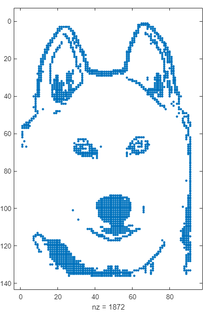
spy
I based my model construction on this PBPK model: PBPK by Armin Sepp. While this is a very convenient script for building a PBPK two-pore model, it's very incovenient for my application to have the species Units defined in molarity. Is there a convenient way to organically switch this model from molarity to grams (or any weight unit)?
We are excited to unveil the ‘Open in MATLAB Online from File Exchange’ feature, which offers MATLAB users a new way to open File Exchange content!
Previously, to experiment with File Exchange code, you were required to download the file and execute it in MATLAB. But now, there's a quicker and easier way to explore the code!
You will find the ‘Open in MATLAB Online’ button next to the ‘Download’ button (see the screenshot below). A simple click transports you directly into the MATLAB Online workflow. It's that straightforward and effortless.
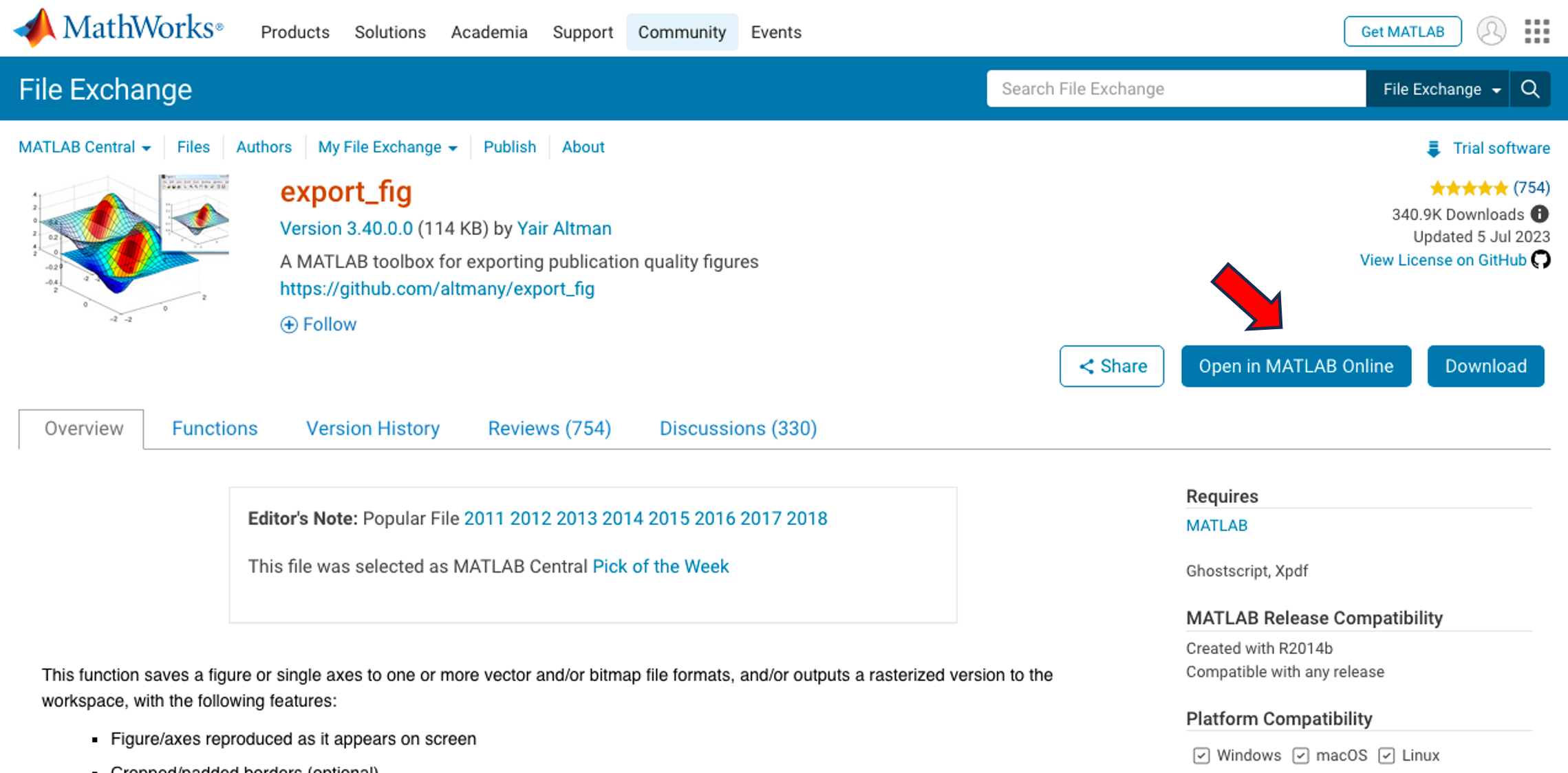
We strongly encourage you to try this new feature. Please share your questions, comments, or ideas by responding to this post!
Hello Community!
We are working on a new translation experience for the MathWorks website and products. The goal is to make it easy for people to see content in the best language for them.
Step 1 is learning from those of you who use another language instead of, or in addition to English. If this sounds like you, we'd love your response to a brief survey.
Feel free to comment here as well. Thanks in advance!
We've released an open-source implementation of STIPA (Speech Transmission Index for Public Address) on GitHub!
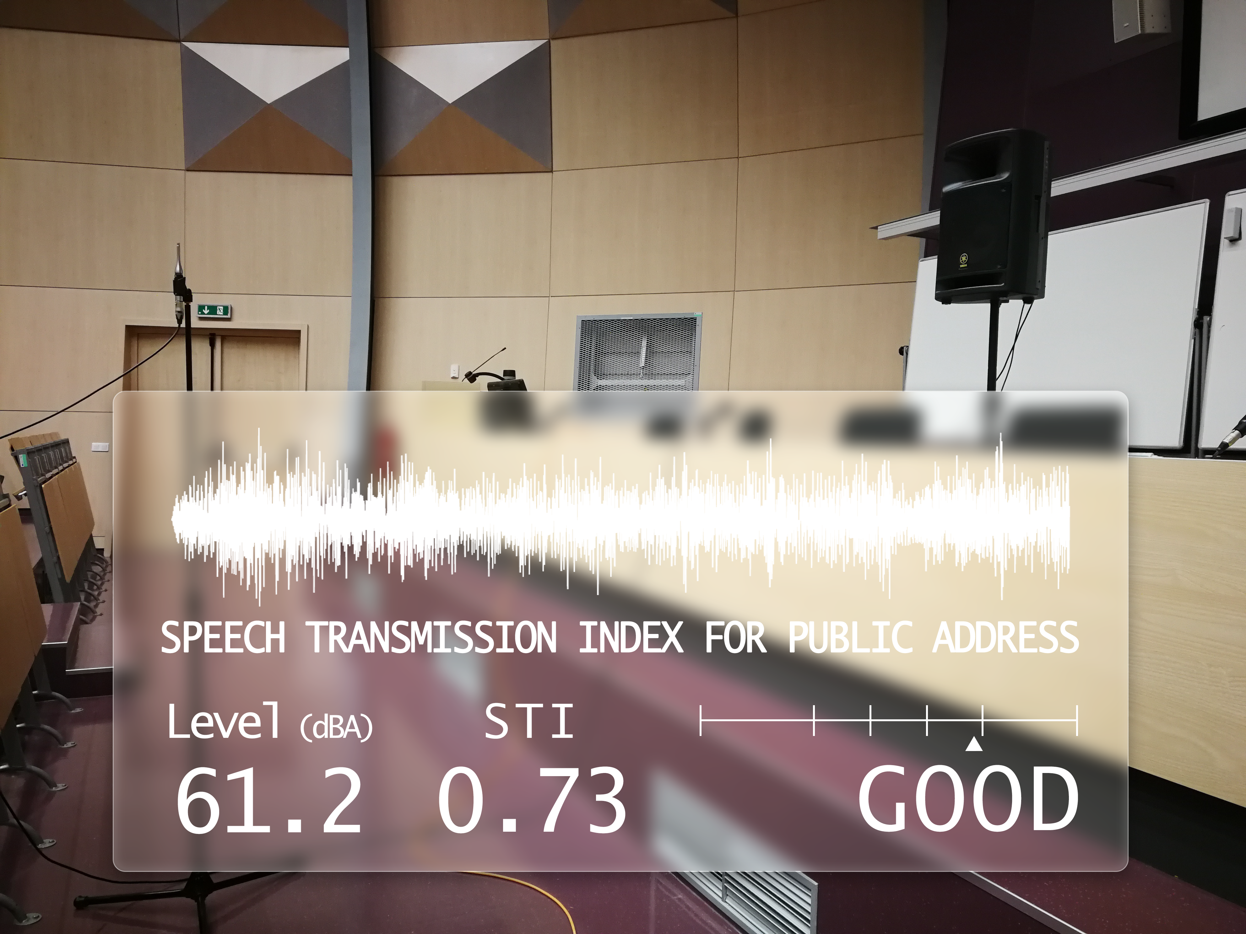
What is STIPA?
Speech Transmission Index is a metric designed to assess the quality of speech transmission through a communication channel. It quantifies the intelligibility of speech signals based on amplitude modulations, providing a standardized measure crucial for evaluating public address systems and communication equipment. STIPA is a version of STI using a simplified measurement method and only one test signal.
Quality Representation:
STI values range from 0 to 1, categorizing speech transmission quality from bad to excellent. The raw STI score can be transformed into the likelihood of intelligibility of syllables, words, and sentences being comprehended.
Verification Tests:
To ensure reliability, we've conducted verification tests according to the IEC 60286-16 standard. Download the test signals and run the stipaVerificationTests.m script from our GitHub repository.
Control Measurements:
We've performed comparative measurements in a university auditorium, showcasing the validity of our implementation.
License:
Our STIPA implementation is distributed under the GNU General Public License 3, reflecting our commitment to open-source collaboration.
I have been finding the AI Chat Playground very useful for daily MATLAB use. In particular it has been very useful for me in basically replacing or supplementing dives into MATLAB documentation. The documentation for MATLAB is in my experience uniformly excellent and thorough but it is sometimes lengthy and hard to parse and the AI Chat is a great one stop shop for many questions I have. However, I would find it very useful if the AI Chat could answer my queries and then also supply a link directly to the documentation. E.g. a box at the bottom of the answer that is basically
"Here is the documentation on the functions AI Chat referred to in this response"
could be neat.
I recently wrote about the new ODE solution framework in MATLAB over the The MATLAB Blog The new solution framework for Ordinary Differential Equations (ODEs) in MATLAB R2023b » The MATLAB Blog - MATLAB & Simulink (mathworks.com)
This was a very popular post at the time - many thousands of views. Clearly everyone cares about ODEs in MATLAB.
This made me wonder. If you could wave a magic wand, what ODE functionality would you have next and why?
Buenas noches. Tengo una estación meteorológica contruida con Arduino, desde hace 4 años y funcionando perfectamente, y veo los datos mediante ThingSpeak. El problema es el que se ve en la imagen:

La méteo, gestionada por una placa Arduino Wemos D1 Mini Pro, una placa solar, una batería y un sensor BME280, funciona cada hora. És decir, está hivernando y cada hora, durante un breve lapso de tiempo, despierta y emite los datos. ThingSpeak los envía a mi ordenador. El problema es que durante 4 años, ha estado enviando, cada hora, una sola lectura de los datos, però ahora envía dos o tres datos con minutos de diferencia, con lo que la lectura y procesamiento de estos datos, se ha vuelto inestable.
No se si es debido a una reinstalación del sistema operativo, debido a un problema que he tenido con el SO, o a qué, pero quisiera volver a ver los datos de forma única, un solo dato cada hora. He sustituido la placa Arduino por otra, pero el problema persiste sin solucionarse, con lo que deduzco que posoblemente deba atribuirse al programa ThingSpeak.
Sería posible solucionar este problema? Hay alguna manera de acceder a modificar, específicamente, esta configuración para volver a mostrar únicamente una lectura por hora?
Gracias por la atención y la ayuda
Salu2 cordiales