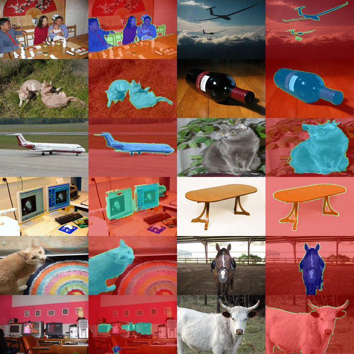
This example shows how to train a semantic segmentation network using deep learning using Pascal VOC dataset.
https://github.com/KentaItakura/Semantic-segmentation-using-Pascal-VOC-with-MATLAB
You are now following this Submission
- You will see updates in your followed content feed
- You may receive emails, depending on your communication preferences
Semantic Segmentation Using Pascal-VOC dataset
[English]
This example shows how to train a semantic segmentation network using deep learning. This example was a modified version of the Matlab official document entitled Semantic Segmentation Using Deep Learning [1]. A semantic segmentation network classifies every pixel in an image, resulting in an image that is segmented by class as shown below.
[Japanese]
この例ではPascal VOCデータセットを用いてセマンティックセグメンテーションを行う例を示します。セマンティックセグメンテーションでは、画像の「塗り絵」のようなことを行い、その領域がどのような物体かを推定します。この例はMATLAB公式ドキュメント [1]をもとに作成しています。下の動画は今回のセグメンテーションの結果の例を示しています。
To illustrate the training procedure, this example trains Deeplab v3+ [2], one type of convolutional neural network (CNN) designed for semantic image segmentation. This example uses the dataset in Visual Object Classes Challenge 2012 (VOC2012) [3]. To run this code, please down load the dataset available at [3].
[1] Semantic Segmentation Using Deep Learning
[2] Chen, Liang-Chieh et al. “Encoder-Decoder with Atrous Separable Convolution for Semantic Image Segmentation.” ECCV (2018).
[3] Visual Object Classes Challenge 2012 (VOC2012)
Load Pascal-VOC Pixel-Labeled Images
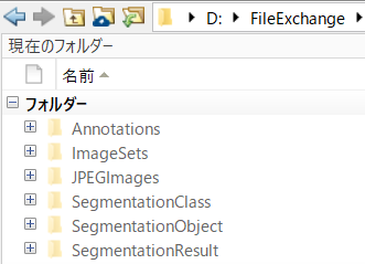
Please run this code after down-loading the Pascal-VOC data from [2]. Unzip and change the directly as shown below. The down-loaded data can be unfrozen into the folders as shown below. The annotated labels were stored in the folder of SegmentationClass. The pixel values in the png images in the Segmentation Class folder corresponds to class ID. Each class ID represents each class.
Use pixelLabelDatastore to load CamVid pixel label image data. A pixelLabelDatastore encapsulates the pixel label data and the label ID to a class name mapping. Use the classes and label IDs to create the pixelLabelDatastore.
clear;clc;close all
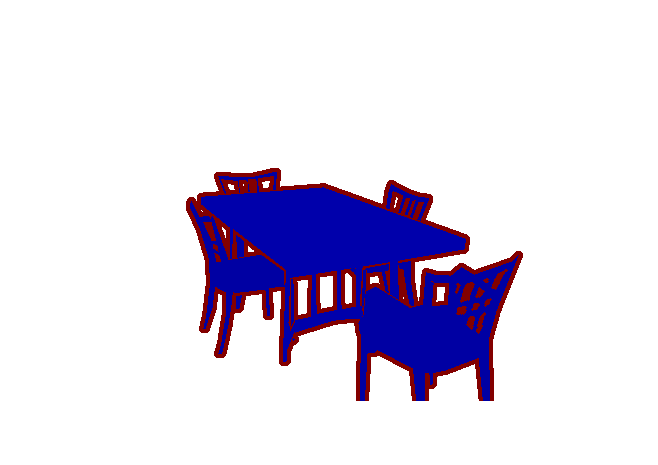
The labeled images are stored in SegmentationClass folder with png format.
labeledImg=imread('./SegmentationClass/2007_003251.png');
The edges have the intensity of 255 while each object ID is like 3, 5, 10. Just using imshow does not depict the labeled image well. Use label2rgb function to convert label matrix into RGB image.
RGB= label2rgb(labeledImg);
figure;imshow(RGB)
Create datastore for images and labels
classes={'background','aeroplane','bicycle','bird','boat','bottle','bus','car','cat','chair','cow','diningtable','dog', ...
    'horse','motorbike','person','potted_plant','sheep','sofa','train','tv_monitor','void'};
labelIDs=[0:20,255];
pxds = pixelLabelDatastore('SegmentationClass',classes,labelIDs);
The RGB image was stored in SegmentationClass folder. The label image and its RGB image can be linked as follows and store the RGB image into image datastore.
imgAddress=strcat(extractBefore(pxds.Files,'SegmentationClass'),'JPEGImages',extractBetween(pxds.Files,'SegmentationClass','png'),'jpg');
imds=imageDatastore(imgAddress);
Display one example
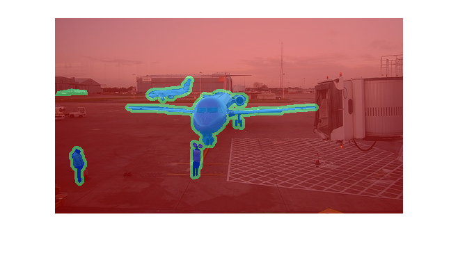
Read and display one of the pixel-labeled images by overlaying it on top of an image.
I = readimage(imds,1);
C = readimage(pxds,1);
B = labeloverlay(I,C);
figure;imshow(B)
Analyze Dataset Statistics
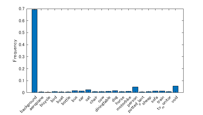
To see the distribution of class labels in the CamVid dataset, use countEachLabel. This function counts the number of pixels by class label.
tbl = countEachLabel(pxds)
| Name | PixelCount | ImagePixelCount | |
|---|---|---|---|
| 1 | 'background' | 361560627 | 519770502 |
| 2 | 'aeroplane' | 3704393 | 30555800 |
| 3 | 'bicycle' | 1571148 | 25999460 |
| 4 | 'bird' | 4384132 | 37509348 |
| 5 | 'boat' | 2862913 | 26733160 |
| 6 | 'bottle' | 3438963 | 33327576 |
| 7 | 'bus' | 8696374 | 27029968 |
| 8 | 'car' | 7088203 | 44884605 |
| 9 | 'cat' | 12473466 | 45464442 |
| 10 | 'chair' | 4975284 | 49342458 |
| 11 | 'cow' | 5027769 | 24278852 |
| 12 | 'diningtable' | 6246382 | 28789770 |
| 13 | 'dog' | 9379340 | 44852930 |
| 14 | 'horse' | 4925676 | 25898409 |
Visualize the pixel counts by class.
frequency = tbl.PixelCount/sum(tbl.PixelCount);

bar(1:numel(classes),frequency)
xticks(1:numel(classes))
xticklabels(tbl.Name)
xtickangle(45)
ylabel('Frequency')
Prepare Training, Validation, and Test Sets
Deeplab v3+ is trained using 80% of the images from the dataset. The rest of the images are split evenly in 10% and 10% for validation and testing respectively. The following code randomly splits the image and pixel label data into a training, validation and test set.
[imdsTrain, imdsVal, imdsTest, pxdsTrain, pxdsVal, pxdsTest] = partitionPascalVOCData(imds,pxds,labelIDs);
Confirm the number of images at each dataset
The 80/10/10 split results in the following number of training, validation and test images:
numTrainingImages = numel(imdsTrain.Files)
numTrainingImages = 2330
numValImages = numel(imdsVal.Files)
numValImages = 291
numTestingImages = numel(imdsTest.Files)
numTestingImages = 292
Create the Network
Use the deeplabv3plusLayers function to create a DeepLab v3+ network based on ResNet-18. The SegNet and U-Net can be used for the semantic segmentation. Please activate the code in this section if you want to try them.
% Specify the network image size. This is typically the same as the traing image sizes.
imageSize = [240 360 3];

% Specify the number of classes.
numClasses = numel(classes);

% Create DeepLab v3+.
lgraph = deeplabv3plusLayers(imageSize, numClasses, 'resnet18');
% lgraph = segnetLayers(imageSize,numClasses,3)
% lgraph = unetLayers(imageSize,numClasses,"EncoderDepth",4);
Specify the class weights using a pixelClassificationLayer.
pxLayer = pixelClassificationLayer('Name','labels','Classes',tbl.Name);
lgraph = replaceLayer(lgraph,'classification',pxLayer);
Data Augmentation
Data augmentation is used during training to provide more examples to the network because it helps improve the accuracy of the network. Here, random left/right reflection and random X/Y translation of +/- 5 pixels is used for data augmentation. Use the imageDataAugmenter to specify these data augmentation parameters.
augmenter = imageDataAugmenter('RandXReflection',false,...
    'RandXTranslation',[-5 5],'RandYTranslation',[-5 5]);
Select Training Options
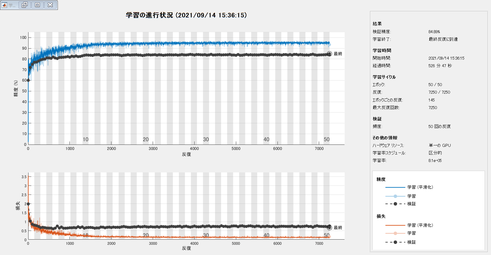
The optimization algorithm used for training is stochastic gradient descent with momentum (SGDM). Use trainingOptions to specify the hyper-parameters used for SGDM.
% Define validation data.
pximdsVal = pixelLabelImageDatastore(imdsVal,pxdsVal,'DataAugmentation',augmenter,'OutputSizeMode',"resize",'OutputSize',[240 360]);

% Define training options.
options = trainingOptions('sgdm', ...% optimizere
    'LearnRateSchedule','piecewise',...% learning rate is reduced every epoch. if you make the rate constant over the traning process, please specify as "none".
    'LearnRateDropPeriod',10,...% reduce the learning rate at the factor of 0.3 every 10 epoch
    'LearnRateDropFactor',0.3,...% reduce the learning rate at the factor of 0.3
    'InitialLearnRate',1e-2, ...% specify initial learning rate
    'L2Regularization',0.0001, ...% L2 regularization
    'ValidationData',pximdsVal,...% validation data
    'MaxEpochs',50, ...% max epoch
    'MiniBatchSize',16, ...% mini-batch size
    'Shuffle','every-epoch', ...% shuffle the data at each epoch
    'VerboseFrequency',500,...% display the training status at every 500 iterations when using trainNetwork
    'Plots','training-progress',...% display the training curve
    'ValidationPatience', Inf); % when the validation accuracy is not decreased for 10 times in a row, training stops
Start Training
Combine the training data and data augmentation selections using pixelLabelImageDatastore. The pixelLabelImageDatastore reads batches of training data, applies data augmentation, and sends the augmented data to the training algorithm.
pximds = pixelLabelImageDatastore(imdsTrain,pxdsTrain, ...
    'DataAugmentation',augmenter,'OutputSizeMode',"resize",'OutputSize',[240 360]);
Training the network
Start training using trainNetwork if the doTraining flag is true. Otherwise, load a pretrained network.
[net, info] = trainNetwork(pximds,lgraph,options);
単一の GPU で学習中。
入力データの正規化を初期化しています。
|===================================================================================|
|  エポック  |  反復  |     経過時間     |  ミニバッチの精度  |  検証精度  |  ミニバッチ損失  |  検証損失  |  基本学習率  |
|        |      |  (hh:mm:ss)  |            |        |           |        |         |
|===================================================================================|
|      1 |    1 |     00:00:47 |      2.41% | 60.06% |    3.5562 | 1.9806 |  0.0100 |
|      1 |   50 |     00:01:51 |     75.74% | 72.12% |    0.8974 | 1.0260 |  0.0100 |
|      1 |  100 |     00:02:51 |     75.60% | 75.05% |    0.7476 | 0.8482 |  0.0100 |
|      2 |  150 |     00:03:52 |     82.04% | 76.96% |    0.5877 | 0.8019 |  0.0100 |
|      2 |  200 |     00:04:51 |     84.26% | 77.12% |    0.4810 | 0.7735 |  0.0100 |
|      2 |  250 |     00:05:48 |     86.52% | 78.17% |    0.4536 | 0.7269 |  0.0100 |
|      3 |  300 |     00:06:46 |     76.89% | 79.19% |    0.7112 | 0.6637 |  0.0100 |
|      3 |  350 |     00:07:46 |     85.05% | 79.74% |    0.4687 | 0.6807 |  0.0100 |
|      3 |  400 |     00:08:44 |     85.
|===================================================================================|
Test Network on One Image
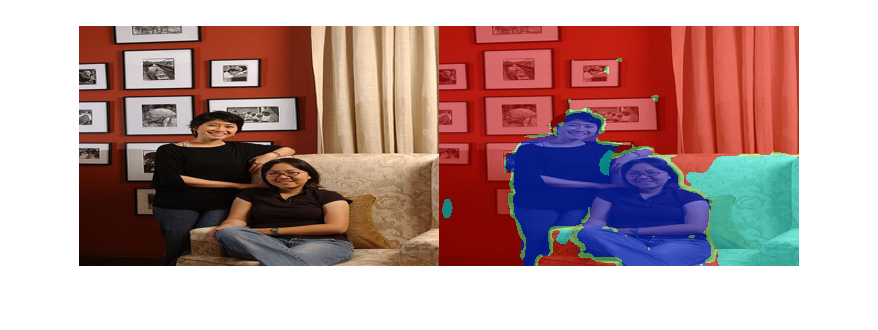
As a quick sanity check, run the trained network on one test image.
I = imresize(readimage(imdsTest,1),[240 360]);
C = semanticseg(I, net);
B = labeloverlay(I,C);
imshowpair(I,B,'montage')
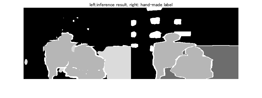
Compare the results in C with the expected ground truth stored in pxdsTest.
expectedResult = read(pxdsTest); pxdsTest.reset
actual = uint8(C);
expected = uint8(imresize(expectedResult{1}, [240 360]));
imshowpair(actual, expected,'montage');title('left:inference result, right: hand-made label')
Visually, the semantic segmentation results overlap well. The amount of overlap per class can be measured using the intersection-over-union (IoU) metric, also known as the Jaccard index. Use the jaccard function to measure IoU.
iou = jaccard(C,imresize(expectedResult{1},size(C)));
table(classes',iou)
| Var1 | iou | |
|---|---|---|
| 1 | 'background' | 0.8681 |
| 2 | 'aeroplane' | NaN |
| 3 | 'bicycle' | NaN |
| 4 | 'bird' | NaN |
| 5 | 'boat' | NaN |
| 6 | 'bottle' | NaN |
| 7 | 'bus' | NaN |
| 8 | 'car' | NaN |
| 9 | 'cat' | NaN |
| 10 | 'chair' | 0 |
| 11 | 'cow' | NaN |
| 12 | 'diningtable' | NaN |
| 13 | 'dog' | NaN |
| 14 | 'horse' | NaN |
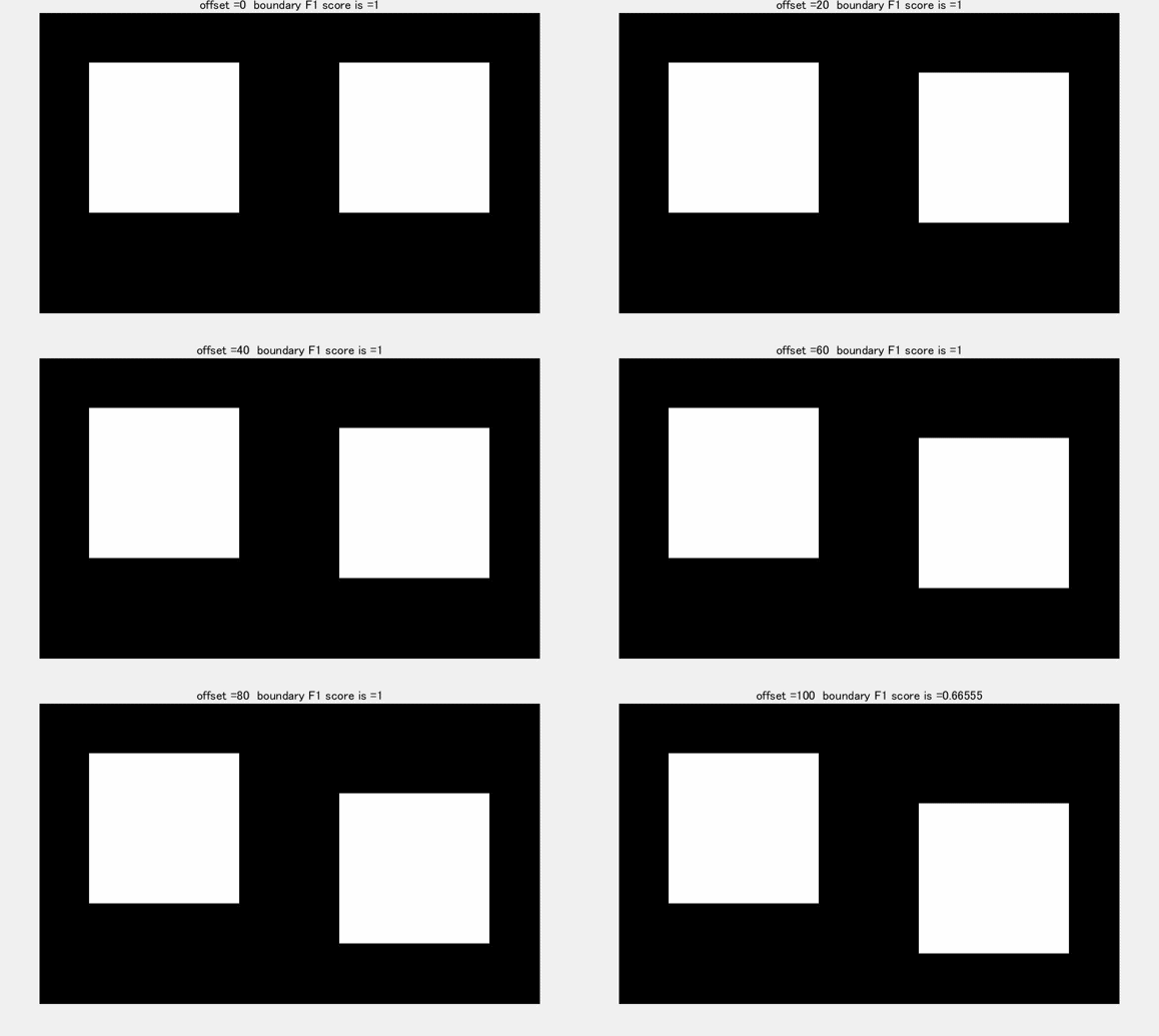
Other common segmentation metrics include the Dice index and the Boundary-F1 contour matching score.
Evaluate Trained Network
To measure accuracy for multiple test images, run semanticseg on the entire test set. A mini-batch size of 10 is used to reduce memory usage while segmenting images. You can increase or decrease this value based on the amount of GPU memory you have on your system. If the GPU memory is not enough, please reduce the value.
Make a folder called SegmentationResult to save the segmentation result.
mkdir SegmentationResult
The segmentation results are saved in the directly specified as [pwd,'\SegmentationResult']. It means, the results are saved in the folder SegmeantationResult in the current directly.
pxdsResults = semanticseg(augmentedImageDatastore([240 360],imdsTest),net, ...
    'MiniBatchSize',10, ...
    'WriteLocation',[pwd,'\SegmentationResult'], ...
    'Verbose',false);
Calculate the semantic segmenation results
Use evaluateSemanticSegmentation to measure semantic segmentation metrics on the test set results.
The labels in pxdsTest are not resized while the size of pxdsResults is 240 by 360 due to the resize function in augmentedImageDatastore. An error is returned when directly comparing the pxdsResults with pxdsTest because the image size is not same; hence the labels in pxdsTest were resized using the read function in the pxdsTest datastore.
pxdsTest.ReadFcn=@(x) imresize(imread(x), [240 360]);
metrics = evaluateSemanticSegmentation(pxdsResults,pxdsTest,'Verbose',false);
evaluateSemanticSegmentation returns various metrics for the entire dataset, for individual classes, and for each test image. To see the dataset level metrics, inspect metrics.DataSetMetrics .
metrics.DataSetMetrics
| GlobalAccuracy | MeanAccuracy | MeanIoU | WeightedIoU | MeanBFScore | |
|---|---|---|---|---|---|
| 1 | 0.8653 | 0.6376 | 0.5350 | 0.7811 | 0.5930 |
The dataset metrics provide a high-level overview of the network performance. To see the impact each class has on the overall performance, inspect the per-class metrics using metrics.ClassMetrics.
metrics.ClassMetrics
| Accuracy | IoU | MeanBFScore | |
|---|---|---|---|
| 1 background | 0.9556 | 0.8825 | 0.8358 |
| 2 aeroplane | 0.6958 | 0.5999 | 0.7193 |
| 3 bicycle | 0.1816 | 0.1286 | 0.3566 |
| 4 bird | 0.8081 | 0.7314 | 0.5103 |
| 5 boat | 0.4481 | 0.3783 | 0.1969 |
| 6 bottle | 0.7337 | 0.6132 | 0.2887 |
| 7 bus | 0.9006 | 0.8101 | 0.5004 |
| 8 car | 0.8049 | 0.6930 | 0.3018 |
| 9 cat | 0.8779 | 0.7335 | 0.4328 |
| 10 chair | 0.2192 | 0.1801 | 0.1480 |
| 11 cow | 0.6441 | 0.5792 | 0.3945 |
| 12 diningtable | 0.5079 | 0.4603 | 0.1947 |
| 13 dog | 0.7714 | 0.6504 | 0.3129 |
| 14 horse | 0.5823 | 0.4313 | 0.2417 |
The animation below shows how BF score works.
Supporting Functions
Deviding the image dataset into training, validation and test data
function [imdsTrain, imdsVal, imdsTest, pxdsTrain, pxdsVal, pxdsTest] = partitionPascalVOCData(imds,pxds,labelIDs)
% Partition CamVid data by randomly selecting 60% of the data for training. The
% rest is used for testing.
numFiles = numel(imds.Files);
shuffledIndices = randperm(numFiles);

% Use 80 % of the images for training.
numTrain = round(0.8 * numFiles);
trainingIdx = shuffledIndices(1:numTrain);

% Use 10 % of the images for validation
numVal = round(0.1 * numFiles);
valIdx = shuffledIndices(numTrain+1:numTrain+numVal);

% Use the rest for testing.
testIdx = shuffledIndices(numTrain+numVal+1:end);

% Create image datastores for training and test.
trainingImages = imds.Files(trainingIdx);
valImages = imds.Files(valIdx);
testImages = imds.Files(testIdx);

imdsTrain = imageDatastore(trainingImages);
imdsVal = imageDatastore(valImages);
imdsTest = imageDatastore(testImages);

% Extract class and label IDs info.
classes = pxds.ClassNames;

% Create pixel label datastores for training and test.
trainingLabels = pxds.Files(trainingIdx);
valLabels = pxds.Files(valIdx);
testLabels = pxds.Files(testIdx);

pxdsTrain = pixelLabelDatastore(trainingLabels, classes, labelIDs);
pxdsVal = pixelLabelDatastore(valLabels, classes, labelIDs);
pxdsTest = pixelLabelDatastore(testLabels, classes, labelIDs);
end
Cite As
Kenta (2026). Semantic segmentation using Pascal VOC (https://github.com/KentaItakura/Semantic-segmentation-using-Pascal-VOC-with-MATLAB/releases/tag/1.1), GitHub. Retrieved .
General Information
- Version 1.1 (4.32 MB)
-
View License on GitHub
MATLAB Release Compatibility
- Compatible with any release
Platform Compatibility
- Windows
- macOS
- Linux
| Version | Published | Release Notes | Action |
|---|---|---|---|
| 1.1 | See release notes for this release on GitHub: https://github.com/KentaItakura/Semantic-segmentation-using-Pascal-VOC-with-MATLAB/releases/tag/1.1 |
||
| 1.0.1 | Japanese description added |
||
| 1.0.0 |


