Top 7 Use Cases for Electric Vehicle Simulation
By Steve Miller, MathWorks
When designing an electric vehicle, engineers need to balance performance and energy efficiency by selecting the right energy storage technology and minimizing powertrain losses. These and other critical tasks require simulation of the physical system throughout development, from selecting a powertrain architecture to testing the embedded software.
This article shows how MATLAB®, Simulink®, and Simscape™ support the seven most common use cases for electric vehicle simulation:
- Explore electric powertrain architectures
- Tune regenerative braking algorithms
- Modify a suspension design
- Optimize vehicle performance
- Develop active chassis controls
- Validate ADAS algorithms
- Test using hardware-in-the-loop (HIL)
The example model used in this article is available for download.
1. Explore Electric Powertrain Architectures
Selecting the right architecture for an electric vehicle design is challenging because of the many options and tradeoffs that must be considered. Architectures can include one, two, or multiple electrical motors; a combustion engine; and various sources of power. Each architecture must be evaluated against criteria such as range, acceleration, performance, and price. Simulation enables you to complete these evaluations by testing candidate architectures on hills and racing circuits and in stop-and-go traffic.
In Simscape, the interfaces between subsystems are physical connections representing mechanical shafts, electrical wires, or fluid in a pipe. The model of the physical system is a schematic that visually communicates how the systems are connected. You can try out various configurations—for example, exchanging a powertrain containing three motors and a battery for a powertrain with a single motor powered by a battery and a fuel cell—and compare the effect of each configuration on vehicle-level performance (Figure 1).

Figure 1. Powertrain configuration options for a Simulink virtual vehicle model.
Tests over different drive cycles and driving styles can be automatically executed, and characteristics such as range and maximum battery temperature can be calculated and compared. This system-level analysis can help you make important decisions, including how large to make the motors and battery, early in the design process.
The simulation results for the three-motor powertrain allow us to compare the effectiveness of two designs for the battery cooling system (Figure 2).
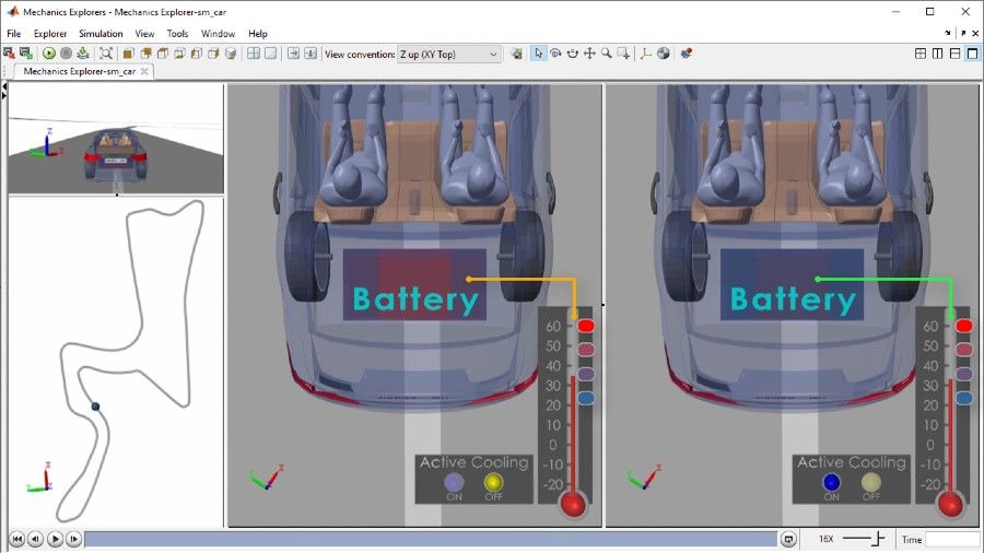
Figure 2. Comparison of battery cooling system designs with different sensor placement.
2. Tune Regenerative Braking Algorithms
A huge advantage of electric vehicles is their ability to recapture kinetic energy and store it in the battery. To maximize the efficiency of this process, the driveline, power converters, and battery design need to be coordinated with the battery management algorithm. In serial regenerative braking, both the regenerative brakes and the conventional brakes are active at the same time, and a control algorithm is required to ensure smooth deceleration.
Simulink models of control algorithms can be connected to Simscape models of brake-by-wire systems that include the hydraulic system and electric motors that generate torque during braking. You can tune both systems to balance requirements for passenger safety and comfort and to maximize the vehicle’s range.
Figure 3 shows a vehicle model configured to use regenerative braking. An algorithm implemented in Simulink determines how much braking torque the electric motors can provide and commands the conventional brakes to provide the remaining required brake torque.
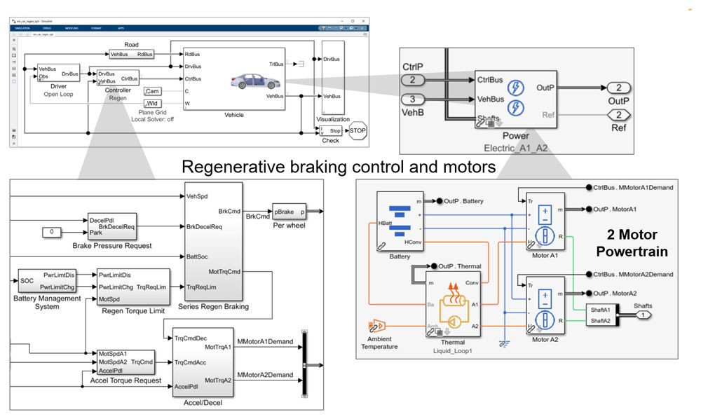
Figure 3. Regenerative braking algorithm integrated with electrical powertrain.
The simulation results show that the algorithm needs to blend the torque provided by each system to enable the vehicle to stop smoothly (Figure 4).
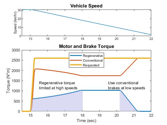
Figure 4. Plot of torque blending during a braking event.
3. Modify Suspension Design
Suspension design involves a tradeoff between passenger comfort and vehicle handling. Suspension behavior depends on a staggering number of parameters, including hardpoint locations, bushing stiffnesses, and spring rates. Simulation helps you tune new designs and test the integration of your component with an existing suspension.
In a Simscape model you can define all these parameters with MATLAB variables and use MATLAB to calculate performance metrics, such as the toe angle of the wheel and the roll center of the vehicle. These parameters can be adjusted automatically until the design meets the requirements.
Figure 5 shows a Simscape model of a vehicle with a multibody suspension. The red spheres represent the hardpoints. These are usually obtained from mechanical designers via the CAD assembly, but can also be measured from an actual vehicle.
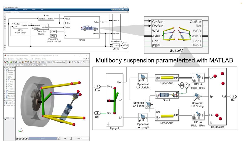
Figure 5. Multibody model of suspension with hardpoints taken from CAD system.
Adjusting the locations of those hardpoints influences the toe and camber curves shown in Figure 6, which will affect vehicle handling.
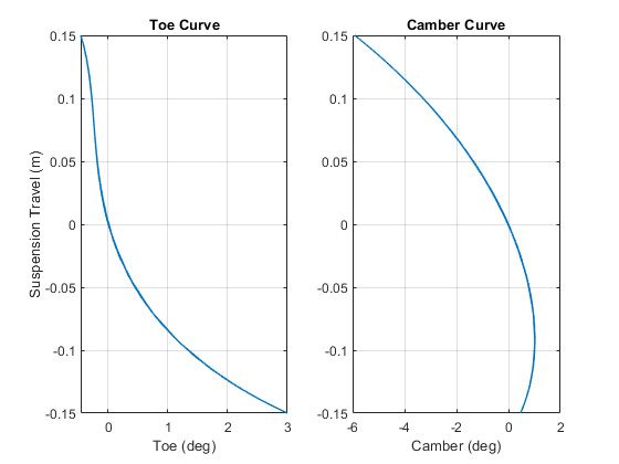
Figure 6. Toe and camber curves for vehicle suspension.
4. Optimize Vehicle-Level Performance
Electric vehicle systems are often developed by several different teams. For example, the mechanical drivetrain and electrical motors are selected by separate teams of engineers and produced by different manufacturers. Braking system algorithms are developed by controls engineers, while the master cylinder, valves, and pumps are selected by hydraulics engineers. For optimal vehicle performance, there must be consistency across these independently developed systems.
Simulation lets you verify that brake caliper pressure, battery capacity, and motor power requirements are in ranges that permit smooth acceleration and deceleration. For example, you can use optimization algorithms in MATLAB to tune the values of these components and to balance lap time and vehicle range.
The plot in Figure 7 shows the result of lap-time optimization. The color of the path around the racetrack indicates the vehicle going faster in the straight sections and slower in the curves, reducing lap time.
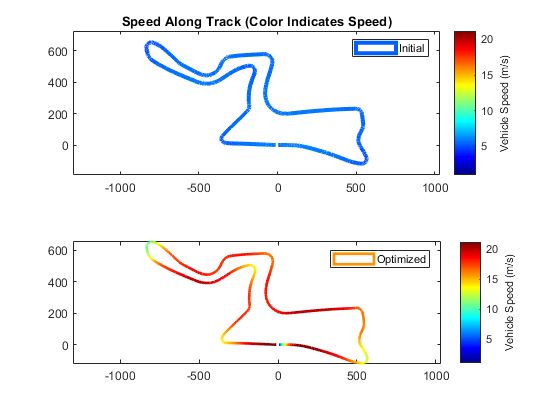
Figure 7. Results of lap-time optimization.
Figure 8 shows that the optimization considered the battery state of charge and temperature as part of its cost function.
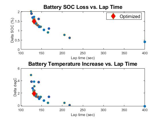
Figure 8. Results of individual iterations of the optimization problem.
5. Develop Active Chassis Controls
Chassis control algorithms such as anti-lock braking, torque vectoring, and electronic stability control are critical safety features. The most challenging physical conditions for these algorithms to operate in, such as driving on icy surfaces or with poorly loaded trailers, are also the most difficult to test.
Simulation enables you to test these extreme cases with no risk to people or equipment. You can include faulty components in the model to ensure that your algorithms are fault tolerant.
The state machine shown in Figure 9 models the logic of an anti-lock brake control system. This logic controls the apply and release valves shown in the hydraulic schematic.
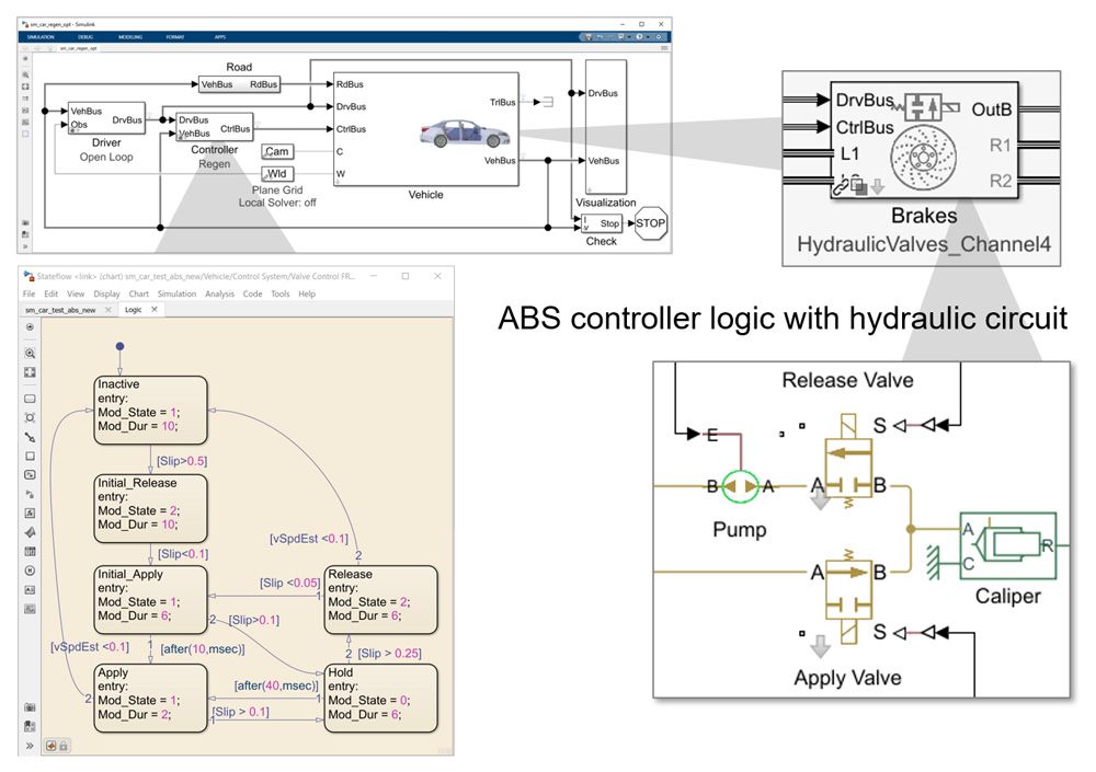
Figure 9. Vehicle model with anti-lock braking algorithm and hydraulic actuation.
The plot in Figure 10 shows how the pressure increases and decreases in steps as the system tries to apply the brakes and keep the wheels spinning.
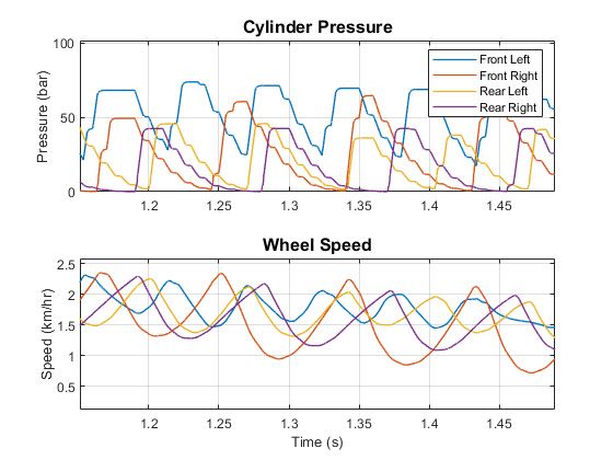
Figure 10. Plot of brake pressure and wheel speed during ABS event.
6. Validate ADAS Algorithms
ADAS algorithms must always meet safety requirements, but the market differentiator might be the quality of the passenger experience. For example, when the vehicle is overtaking, the algorithm may use harsh steering and braking maneuvers that throw the passengers off balance. Subjective qualities like passenger comfort are difficult to evaluate. But a simulation model can produce measurements that let you quantify passenger discomfort levels.
You can model passengers as 3D mechanical humanoids with joints and instrument them with accelerometers to capture the acceleration and jerk that passengers feel as the vehicle moves through a maneuver guided by an ADAS algorithm. You can then postprocess the accelerometer data in MATLAB to derive an index of discomfort.
Figure 11 shows a vehicle model with 3D mechanical models of the passengers. In the simulation we test an ADAS algorithm by following a path through a test facility.
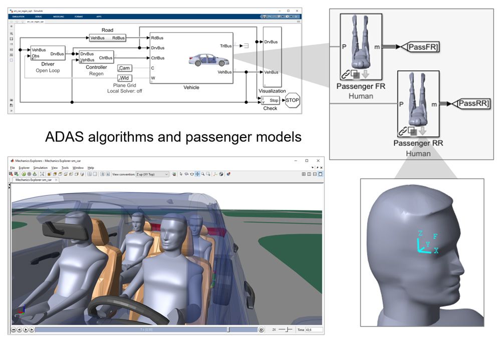
Figure 11. Vehicle model with multibody models of passengers.
Figure 12 shows the simulation results. We can see that the vehicle pitches forward sharply during one portion of the maneuver due to the algorithm’s decision to apply the brakes.
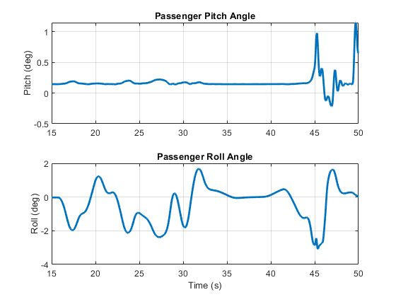
Figure 12. Plot of passenger motion during a test of ADAS algorithms.
7. Test Using Hardware-in-the-Loop
Embedded control software must react appropriately when exposed to experienced or naïve drivers, icy streets, or abrupt maneuvers in new or old vehicles. It is impractical to test every combination of factors in an actual vehicle. With simulation, you can test embedded control software in a virtual vehicle.
You can convert Simscape models to C code and use those models in HIL tests. HIL lets you test the embedded control unit (hardware and software) in real-time simulation with any type of vehicle and under any conditions, including worst-case scenarios such as overheated batteries and short-circuited electrical networks.
Figure 13 shows the execution time per time step in an HIL test. This model was run on Speedgoat hardware using Simulink Real-Time™, but it could also be run on other real-time simulation hardware.
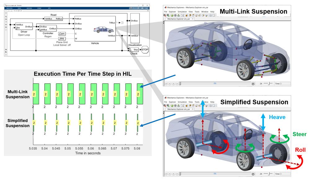
Figure 13. Execution time in an HIL test for two configurations of a vehicle model.
The fidelity level of the suspension model can be adjusted to leave more execution time per time step for other computational tasks.
Summary
With the technology used in electric vehicles advancing rapidly, it is critical to assess the effect of introducing these technologies into your design. A flexible, configurable simulation model can enable you to explore these and other tradeoffs rapidly, without risk, and at every stage of the development process.
Published 2021
View Articles for Related Capabilities
View Articles for Related Industries
Select a Web Site
Choose a web site to get translated content where available and see local events and offers. Based on your location, we recommend that you select: United States.
You can also select a web site from the following list
Americas
- América Latina (Español)
- Canada (English)
- United States (English)
Europe
- Belgium (English)
- Denmark (English)
- Deutschland (Deutsch)
- España (Español)
- Finland (English)
- France (Français)
- Ireland (English)
- Italia (Italiano)
- Luxembourg (English)
- Netherlands (English)
- Norway (English)
- Österreich (Deutsch)
- Portugal (English)
- Sweden (English)
- Switzerland
- United Kingdom (English)