Introduction to TR 38.901 ISAC Channel Model

Since R2026a

This example shows how to create, configure, and simulate the TR 38.901 integrated sensing and communication (ISAC) channel model [1].

Introduction

The 3GPP TR 38.901 ISAC channel model is a geometry-based stochastic channel between a sensing transmitter, one or more sensing targets, and a sensing receiver. The model extends the TR 38.901 spatial channel model (SCM). The channel output is the superposition of a background channel (multipath propagation between STX and SRX through the environment) and a target channel (reflections from sensing targets). This combined output enables simulation of systems where the same waveform is used for both communication and sensing.

Create a Bistatic ISAC Scenario

To simulate TRP-UE bistatic sensing of a UAV target, create and configure an h38901ISACChannel System object. In this mode, a base station (TRP) acts as the sensing transmitter and a user equipment (UE) acts as the sensing receiver. The channel supports six sensing modes: TRP Monostatic, UE Monostatic, TRP-UE Bistatic, UE-TRP Bistatic, TRP-TRP Bistatic, and UE-UE Bistatic.

Set the random number generator to its default state for reproducibility.

rng("default");
channel = h38901ISACChannel;
channel.SensingMode = "TRP-UE Bistatic";
channel.SensingScenario = "ISAC-UAV";
channel.CommunicationScenario = "UMi";
channel.CenterFrequency = 28e9;

Configure the Nodes

The channel has three types of nodes: the sensing transmitter (STX), sensing targets (STs), and the sensing receiver (SRX). Configure their positions and antenna arrays as appropriate.

Antenna arrays can be configured in three ways:

1. NumTransmitAntennas or NumReceiveAntennas - a convenience property that creates a default panel array.

2. A structure with fields Size, ElementSpacing, PolarizationAngles, Element, and PolarizationModel - the same format as the TransmitAntennaArray property of nrCDLChannel.

3. A Phased Array System Toolbox antenna object (for example, phased.ULA).

This example uses NumTransmitAntennas and NumReceiveAntennas for simplicity. Set up the sensing transmitter (base station) at a height of 10 m with four antenna elements. Point the transmit array normal along the x-axis. The TransmitArrayOrientation vector specifies the bearing, downtilt, and slant rotation angles in degrees, respectively, as specified in TR 38.901 Section 7.1.3.

channel.STX.Position = [0; 0; 10]; % [x; y; z] (m)
channel.STX.NumTransmitAntennas = 4;
channel.STX.TransmitArrayOrientation = [0; 0; 0]; % [bearing; downtilt; slant] (degrees)

Set up the sensing receiver (UE) at 80 m distance. Point the receive array normal along the negative y-axis.

channel.SRX.Position = [60; 50; 1.5];
channel.SRX.NumReceiveAntennas = 4;
channel.SRX.ReceiveArrayOrientation = [270; 0; 0]; % [bearing; downtilt; slant] (degrees)

Configure a sensing target with a position, velocity, and orientation. The SensingScenario property (set above to "ISAC-UAV") determines the target type and its associated radar cross section (RCS) and propagation statistics - the STs structure defines only the target's geometry and motion.

channel.STs.Position = [50; 20; 15];  % [x; y; z] (m)
channel.STs.Velocity = [5; 3; 0];     % [x; y; z] (m/s)
channel.STs.Orientation = [0; 0; 0];  % [bearing; downtilt; slant] (degrees)

Set additional channel properties.

channel.SampleRate = 30.72e6;
channel.Seed = 42;

Visualize the Scenario

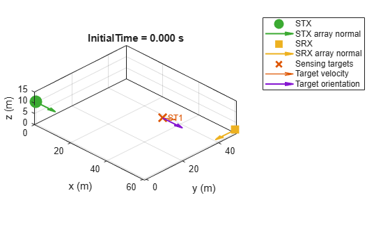
To verify that array orientations point toward the sensing targets, use the displayChannel object function to plot the node positions and antenna array normal vectors. This is a useful sanity check to verify that the array orientations point toward the region of interest (the sensing targets).

figure;
displayChannel(channel);

Channel Composition

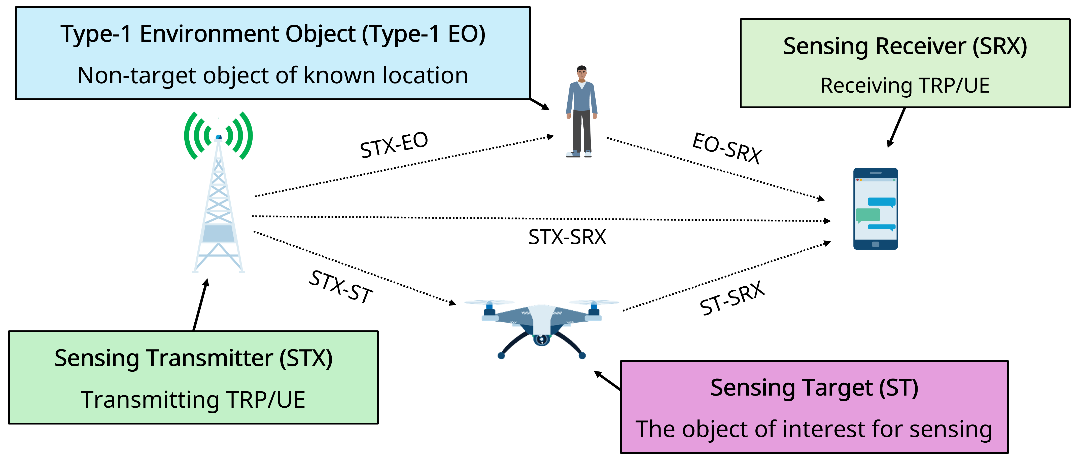
The diagram shows the key elements of the ISAC channel model. The STX and SRX communicate through the environment. A ST is represented by one or more scattering points of the sensing target (SPSTs). The ST reflects signals from the transmitter toward the receiver. Type-1 environment objects (EOs) are static scatterers that produce additional reflections through two-stage STX-EO and EO-SRX propagation links. EOs are modeled as additional sensing targets in the STs array with the same RCS models as other targets. They typically have zero velocity to represent stationary environmental clutter.

The ISAC channel output is the superposition of the background and target channel components:

• Background channel: models multipath propagation between STX and SRX directly. The background channel generates clutter that sensing algorithms must suppress.

• Target channel: models the two-stage propagation path from STX to the SPSTs, and from the SPSTs to SRX. Each stage independently undergoes TR 38.901 Section 7.9.4 Steps 9-15 (ray generation, coupling, antenna response, and Doppler). A RCS model is applied at the target to determine the amplitude and phase of reflected paths. The target paths carry the sensing information (range, velocity, and angle of targets).

The BackgroundChannel and TargetChannel properties control which components are included in the output. You can use them to experiment with the channel. Both are enabled by default to produce the combined channel. Force LOS for the target channel so that the direct path is always present, making it easier to visualize. Set ChannelFiltering to false to generate path gains without passing a waveform.

channel.TargetChannel = true;
channel.BackgroundChannel = true;
channel.LOSProbability = 1;
channel.ChannelFiltering = false;
channel.NumTimeSamples = 1;

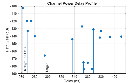
Generate the combined channel path gains and sample times for the background and target channels. Paths at the same delays are combined for efficiency.

[pathGains, sampleTimes] = channel();

The info object function returns the UniquePathDelays.

channelInfo = info(channel);
disp("Number of combined path gains: " + width(pathGains))

Number of combined path gains: 17

Compute the expected propagation delays from the scenario geometry. The background LOS delay corresponds to the direct STX-to-SRX distance, and the target delay corresponds to the two-leg path STX-to-ST-to-SRX.

[expectedTargetDelay, expectedBackgroundLOSDelay] = bistaticDelays(channel);

Plot the power delay profile with expected component delays.

figure;
plotPDP(channelInfo.UniquePathDelays,pathGains,"Background");
xline(expectedBackgroundLOSDelay*1e9, "--", "Background LOS", LabelVerticalAlignment="bottom", DisplayName="Expected delay");
xline(expectedTargetDelay*1e9, "--", "Target", LabelVerticalAlignment="bottom", HandleVisibility="off");
xlabel("Delay (ns)");
ylabel("Path Gain (dB)");
title("Channel Power Delay Profile");
grid on;

Visualize Channel Components

The info object function returns PathGains and PathDelays as cell arrays. The first cell contains the background channel contribution and subsequent cells contain the target channel links. This allows you to evaluate the contributions of different sources.

disp("Number of links: " + numel(channelInfo.PathGains))

Number of links: 2

disp("Background paths: " + size(channelInfo.PathGains{1}, 2))

Background paths: 17

disp("Target paths: " + size(channelInfo.PathGains{2}, 2))

Target paths: 5

Plot the power delay profile showing the background and target channel components overlaid. The background paths cluster around the direct LOS delay while the target path aligns with the two-leg STX-to-ST-to-SRX propagation delay. Note that the target path powers are lower than the background paths.

bgPathGains = channelInfo.PathGains{1};
bgDelays = channelInfo.PathDelays{1};
tgtPathGains = channelInfo.PathGains{2};
tgtDelays = channelInfo.PathDelays{2};
figure
hold on;
plotPDP(bgDelays,bgPathGains,"Background");
plotPDP(tgtDelays,tgtPathGains,"Target");
xline(expectedBackgroundLOSDelay*1e9, "--", "Background LOS", LabelVerticalAlignment="bottom", DisplayName="Expected delay");
xline(expectedTargetDelay*1e9, "--", "Target", LabelVerticalAlignment="bottom", HandleVisibility="off");
hold off;
xlabel("Delay (ns)");
ylabel("Path Gain (dB)");
title("Channel Power Delay Profile");
legend;
grid on;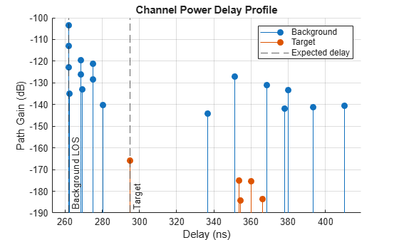

Compare Sensing Modes: Bistatic vs. Monostatic

The channel supports both bistatic and monostatic sensing modes. In bistatic modes, separate nodes transmit and receive. In monostatic modes, the same node transmits and receives, sensing targets through the radar echo. A key difference between monostatic and bistatic modes is how the background channel is generated.

In bistatic modes, the background is a standard TR 38.901 channel between the physically separated STX and SRX, producing a single set of background paths.

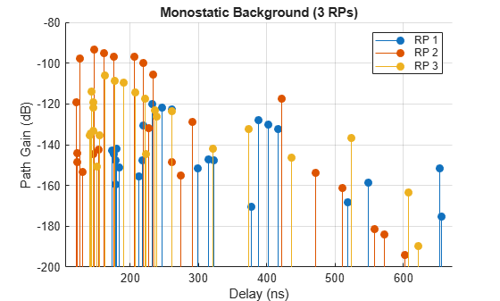
In monostatic modes, the STX and SRX are co-located so there is no meaningful propagation geometry between them. Instead, the channel generates three virtual reference points at random positions around the monostatic node, spaced 120 degrees apart in azimuth. The model generates a separate NLOS channel between the node and each RP. The superposition of these three channels models the round-trip scattering environment that a monostatic radar experiences.

Create a monostatic scenario. The STX and SRX must be co-located (same position, velocity, orientation, and size).

monoChannel = h38901ISACChannel;
monoChannel.SensingMode = "TRP Monostatic";
monoChannel.SensingScenario = "ISAC-UAV";
monoChannel.CommunicationScenario = "UMi";
monoChannel.STX.Position = [0; 0; 10];
monoChannel.STX.Orientation = [0; 0; 0];
monoChannel.STX.NumTransmitAntennas = 4;
monoChannel.SRX.Position = [0; 0; 10];
monoChannel.SRX.Orientation = [0; 0; 0];
monoChannel.SRX.NumReceiveAntennas = 4;
monoChannel.STs.Position = [30; 20; 15];
monoChannel.STs.Velocity = [5; 3; 0];
monoChannel.ChannelFiltering = false;

Generate path gains for the monostatic channel.

[monoPathGains, monoSampleTimes] = monoChannel();
monoInfo = info(monoChannel);

The info object function returns path gains and delays as a cell array of links. The structure is:

• Bistatic modes: 2 links (1 background link + 1 target link).

• Monostatic modes: 4 links. The 3-RP method produces 3 background links (one per reference point) + 1 target link.

Plot the monostatic background power delay profile to see the three reference point channels.

figure;
hold on;
for i = 1:3
    plotPDP(monoInfo.PathDelays{i},monoInfo.PathGains{i},"RP "+i);
end
hold off;
xlabel("Delay (ns)");
ylabel("Path Gain (dB)");
title("Monostatic Background (3 RPs)");
legend;
grid on;

Configure Sensing Targets

The STs structure defines the geometry, motion, and physical characteristics of each sensing target. The SensingScenario property determines the target type and its associated RCS and propagation statistics.

Sensing Scenarios

This table summarizes the four scenarios and their compatibility with RCS models and supported communication scenarios.

Sensing Scenario	Target Type	RCS Model 1	RCS Model 2	Communication Scenarios
ISAC-UAV	Unmanned aerial vehicle	Yes	Yes	UMi, UMa, RMa (and AV variants)
ISAC-Human	Human	Yes	Yes	UMi, UMa, RMa, InH, InF variants
ISAC-AGV	Automated guided vehicle	No	Yes	InF variants only
ISAC-Automotive	Road vehicle	No	Yes	UMi, UMa, RMa

The SensingScenario property affects the RCS statistics used in the target channel but does not change the background channel, which is governed by the CommunicationScenario property.

RCS Model and Sensing Target Scattering Points

The RCSModel property controls how the target's RCS is represented:

• Model 1: Single scattering point with angle-independent RCS. Available for ISAC-UAV and ISAC-Human only.

• Model 2: Angular-dependent RCS. For example, a vehicle's broadside returns more energy than its front. Available for all sensing scenarios and required for ISAC-AGV and ISAC-Automotive.

When using Model 2, the MultipleSPSTs flag controls whether the target has one or five scattering points (SPSTs):

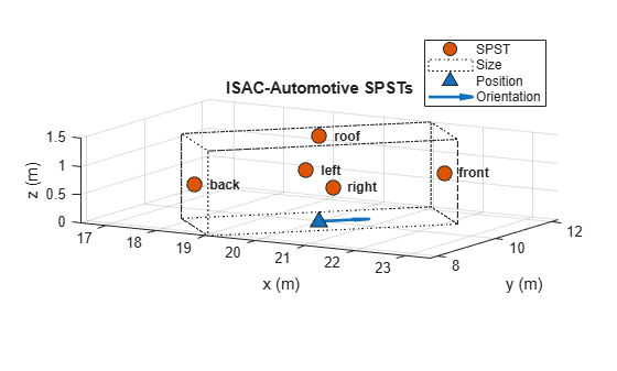
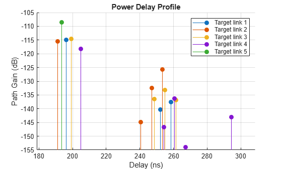
• MultipleSPSTs = false (default): A single scattering point.

• MultipleSPSTs = true: Five scattering points placed at the front, left, back, right, and roof of the target (positions determined by Size). Each produces its own path delays, so the target's physical extent is visible in the channel impulse response. Only valid for ISAC-Automotive and ISAC-AGV.

Position, Size, Velocity, and Orientation

Each sensing target has the following motion and geometry fields:

• Position: [x y z] in meters. For vehicles, AGVs, and humans, this is the ground-contact reference point (center of the footprint at ground level).

• Size: [L W H] vector specifying the target's physical extent in meters (length, width, height).

• Velocity: [vx vy vz] in m/s - introduces Doppler shifts on target paths.

• Orientation: [bearing; downtilt; slant] in degrees. This rotation affects both the angular RCS pattern and the physical placement of scattering points. A bearing of 0° means the target's front faces the positive x-axis.

The model places SPSTs on or around the target reference Position using offsets derived from Size depending on the SensingScenario and MultipleSPSTs

SPSTs are placed at offsets from Position in the target's local coordinate system (LCS), then rotated into the global coordinate system by Orientation. The offsets depend on the sensing scenario:

Sensing Scenario	SPST Offsets from Position (LCS)	Notes
ISAC-Automotive / ISAC-AGV (MultipleSPSTs=true)	Front: (L/2, 0, H/2), Left: (0, W/2, H/2), Back: (-L/2, 0, H/2), Right: (0, -W/2, H/2), Roof: (0, 0, H)	Five independent SPSTs with distinct path delays
ISAC-Automotive / ISAC-AGV (MultipleSPSTs=false)	Center: (0, 0, H/2)	Single SPST at half-height above ground
ISAC-Human	Torso: (0, 0, scaled to 1.5 m)	Height scaled relative to 1.75 m reference adult
ISAC-UAV	None: (0, 0, 0)	Position is used directly as the SPST location

Configure an automotive sensing scenario with multiple SPSTs.

model2Chan = h38901ISACChannel;
model2Chan.SensingMode = "TRP-UE Bistatic";
model2Chan.SensingScenario = "ISAC-Automotive";
model2Chan.RCSModel = "Model 2";
model2Chan.CommunicationScenario = "UMi";
model2Chan.SRX.Position = [10; 10; 25];
model2Chan.STs.Position = [20; 10; 0];
model2Chan.STs.Velocity = [5; 3; 0];
model2Chan.STs.Size = [4.5 1.8 1.5]; % sedan: 4.5 m long, 1.8 m wide, 1.5 m tall
model2Chan.STs.Orientation = [45; 0; 0];
model2Chan.STs.MultipleSPSTs = true;
model2Chan.ChannelFiltering = false;

Visualize the physical placement of the five SPSTs on the vehicle in the global coordinate system.

figure;
displaySPSTs(model2Chan);

Inspect the five target links produced by multiple SPSTs.

model2Chan();
rcsInfo = info(model2Chan);
tgtOffset = 2; % First path is background
figure;
hold on;
for i = tgtOffset:numel(rcsInfo.PathDelays)
    plotPDP(rcsInfo.PathDelays{i},rcsInfo.PathGains{i},"Target link "+(i-1));
end
hold off;
xlabel("Delay (ns)");
ylabel("Path Gain (dB)");
title("Power Delay Profile");
legend;
grid on;

Multiple Sensing Targets

The channel supports multiple sensing targets.

mtChannel = h38901ISACChannel;
mtChannel.SensingMode = "TRP-UE Bistatic";
mtChannel.SensingScenario = "ISAC-UAV";
mtChannel.CommunicationScenario = "UMi";
mtChannel.CenterFrequency = 28e9;
mtChannel.STX.Position = [0; 0; 10];
mtChannel.STX.NumTransmitAntennas = 4;
mtChannel.STX.TransmitArrayOrientation = [0; 0; 0];
mtChannel.SRX.Position = [60; 50; 1.5];
mtChannel.SRX.NumReceiveAntennas = 4;
mtChannel.SRX.ReceiveArrayOrientation = [180; 0; 0];
mtChannel.SampleRate = 30.72e6;
mtChannel.ChannelFiltering = false;
mtChannel.LOSProbability = 1;
mtChannel.Seed = 42;

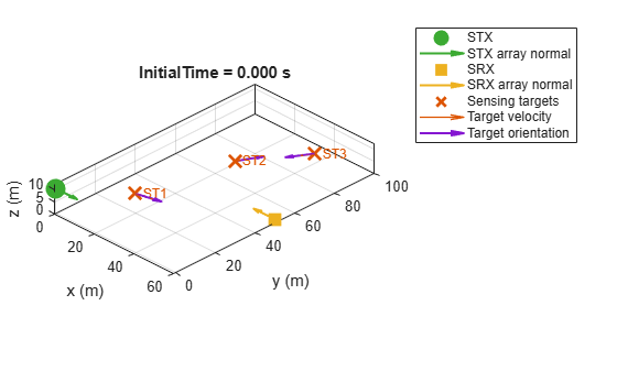
Expand STs to a structure array, with each element defining an independent sensing target. Define each target.

mtChannel.STs = repmat(mtChannel.STs, 1, 3);
mtChannel.STs(1).Position = [25; 15; 12];
mtChannel.STs(1).Velocity = [8; 2; 0];
mtChannel.STs(1).Orientation = alignOrientationWithVelocity(mtChannel.STs(1).Velocity);

mtChannel.STs(2).Position = [30; 60; 9];
mtChannel.STs(2).Velocity = [1; 2; 0];
mtChannel.STs(2).Orientation = alignOrientationWithVelocity(mtChannel.STs(2).Velocity);

mtChannel.STs(3).Position = [45; 85; 8];
mtChannel.STs(3).Velocity = [-3; -5; 0];
mtChannel.STs(3).Orientation = alignOrientationWithVelocity(mtChannel.STs(3).Velocity);

figure;
displayChannel(mtChannel);

[mtPathGains, mtSampleTimes] = mtChannel();
mtInfo = info(mtChannel);

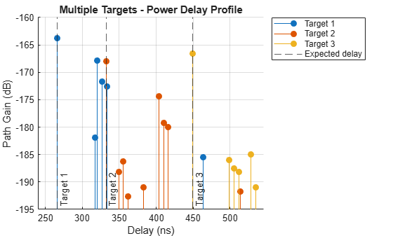
Each target produces its own target link in the output. Visualize the path delays for each target separately.

disp("Total links: " + numel(mtInfo.PathGains) + " (1 background + " + (numel(mtInfo.PathGains)-1) + " target)")

Total links: 4 (1 background + 3 target)

expectedTargetDelay = bistaticDelays(mtChannel);
figure;
hold on;
for i = 2:numel(mtInfo.PathDelays)
    plotPDP(mtInfo.PathDelays{i},mtInfo.PathGains{i},"Target "+(i-1));
    l = xline(expectedTargetDelay(i-1)*1e9, "--", "Target "+(i-1), LabelVerticalAlignment="bottom", HandleVisibility="off");
end
l.HandleVisibility = "on";
l.DisplayName = "Expected delay";
hold off;
xlabel("Delay (ns)");
ylabel("Path Gain (dB)");
title("Multiple Targets - Power Delay Profile");
legend(Location="bestoutside");
grid on;

Moving Targets

Model a scenario with a moving target and track it over time.

movingChannel = h38901ISACChannel;
movingChannel.SensingMode = "TRP Monostatic";
movingChannel.SensingScenario = "ISAC-UAV";
movingChannel.CommunicationScenario = "UMi";
movingChannel.CenterFrequency = 28e9;
movingChannel.STX.Position = [-10; -10; 10];
movingChannel.STX.NumTransmitAntennas = 1;
movingChannel.STX.TransmitArrayOrientation = [90; 0; 0];
movingChannel.SRX.Position = [-10; -10; 10];
movingChannel.SRX.NumReceiveAntennas = 1;
movingChannel.SRX.ReceiveArrayOrientation = [90; 0; 0];
movingChannel.STs.Position = [-20; -10; 5];
movingChannel.STs.Velocity = [3; 4; 0.1];
movingChannel.STs.Orientation = alignOrientationWithVelocity(movingChannel.STs.Velocity);
movingChannel.SampleRate = 30.72e6;
movingChannel.ChannelFiltering = false;
movingChannel.LOSProbability = 1;
movingChannel.Seed = 42;
movingChannel.ThresholdPower = -25;

Each call of the channel models a block of time starting at InitialTime. The block duration is NumTimeSamples / SampleRate when ChannelFiltering is disabled, or the input waveform duration when ChannelFiltering is enabled. Within a block for STX, SRX and STs, Velocity drives Doppler response, and Position is the position for the duration of the block. The channel does not advance position internally with time. To simulate a moving target across multiple blocks, update InitialTime to the start of each block and advance STs.Position externally to match.

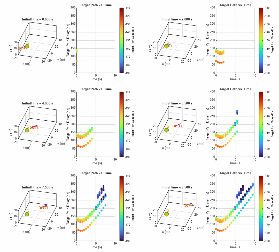
Simulate 20 blocks separated by 0.5 seconds. Set NumTimeSamples to 1 so that each block produces a single snapshot. Plot the scenario and path delay scatter side by side at each time step. The number of path gains changes over time due to the stochastic process and weak path filtering based on the ThresholdPower property.

dt = 0.5; % seconds
numBlocks = 20;
movingChannel.NumTimeSamples = 1;

[ax3d, axScatter] = setupMotionPlot(numBlocks,dt);
displayChannel(movingChannel, ax3d, XLim=[-20 20], YLim=[-20 40], ZLim=[0 20], Legend="off");
view(ax3d, 15, 30);
for b = 1:numBlocks
    movingChannel.InitialTime = (b-1)*dt;
    movingChannel.STs.Position = movingChannel.STs.Position+movingChannel.STs.Velocity*dt*(b>1);
    movingChannel();
    displayChannel(movingChannel, ax3d);
    frameInfo = info(movingChannel);
    tgtDelays = frameInfo.PathDelays{end}*1e9;
    tgtPGs = frameInfo.PathGains{end};
    scatter(axScatter, movingChannel.InitialTime*ones(numel(tgtDelays),1), tgtDelays.', 36, mag2db(abs(tgtPGs)).', "filled");
    drawnow;
end

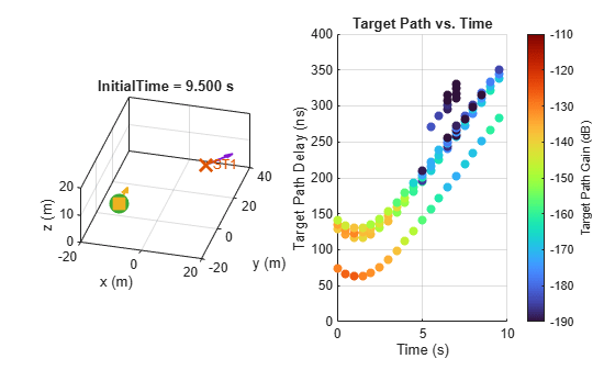
This is the resulting animation.

Channel Filtering with a Waveform

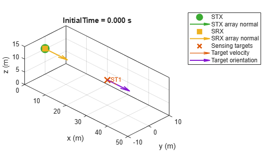
In this section, pass a waveform through the channel and create a range-Doppler map to detect a target. To pass a signal through the channel, set ChannelFiltering to true and provide a transmit waveform. Reconfigure the monostatic channel for UAV sensing with filtering enabled. Disable the background channel and increase the carrier frequency to 28 GHz so the target Doppler is clear.

release(monoChannel);
monoChannel.STX.NumTransmitAntennas = 1;  
monoChannel.STX.TransmitArrayOrientation = [0; 0; 0];
monoChannel.SRX.NumReceiveAntennas = 1;
monoChannel.SRX.ReceiveArrayOrientation = [0; 0; 0];
monoChannel.STs.Position = [30; 0; 10];
monoChannel.STs.Velocity = [5; 0; 0];

monoChannel.CenterFrequency = 28e9;
monoChannel.ChannelFiltering = true;
monoChannel.BackgroundChannel = false;
monoChannel.LOSProbability = 1;
figure;
displayChannel(monoChannel, YLim=[-10 10], ZLim=[0 15]);

Create a phase-coded (PMCW) waveform.

numPulses = 512;
waveform = phased.PhaseCodedWaveform( ...
    SampleRate=monoChannel.SampleRate, ...
    NumChips=256, ...
    ChipWidth=1/monoChannel.SampleRate, ...
    PRF=60e3, ...
    NumPulses=numPulses);
numPulseSamples = monoChannel.SampleRate/waveform.PRF;
txWaveform = waveform();

Pass consecutive pulses through the channel. For simplicity do not update the initial time or target position for each pulse.

rxWaveform = monoChannel(txWaveform);

Synchronize the waveform. Remove channel filter implementation delay so the measured delay is only due to the target range.

cfDelay = info(monoChannel).ChannelFilterDelay;
rxWaveform = rxWaveform(cfDelay+1:end);

Create matrix of a receive pulse per column.

rxPulses = reshape(rxWaveform(1:numPulseSamples*(numPulses-1)),numPulseSamples,numPulses-1);

Compute and plot the range-Doppler response. The moving target appears as a peak offset from zero Doppler at its monostatic range.

rdResp = phased.RangeDopplerResponse( ...
    RangeMethod="Matched filter", ...
    SampleRate=monoChannel.SampleRate, ...
    OperatingFrequency=monoChannel.CenterFrequency, ... 
    DopplerOutput="Speed");
figure;
plotResponse(rdResp, rxPulses, getMatchedFilter(waveform));
ylim([0 200]);
xlim([-10 10]);

Overlay the expected target range and Doppler computed from the monostatic geometry and velocity.

hold on
plotExpectedTargetMonostaticRDR(monoChannel,DopplerOutput=rdResp.DopplerOutput);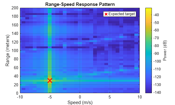

For a full end-to-end ISAC workflow demonstrating target detection and tracking using 5G NR waveforms, see the Integrated Sensing and Communication Using 5G Waveform (Phased Array System Toolbox) example.

References

[1] 3GPP TR 38.901. “Study on channel model for frequencies from 0.5 to 100 GHz.” 3rd Generation Partnership Project; Technical Specification Group Radio Access Network.

Local Functions

function [targetDelay,losDelay] = bistaticDelays(channel)
    c = physconst("LightSpeed");
    dSTX_SRX = norm(channel.SRX.Position-channel.STX.Position);
    losDelay = dSTX_SRX./c;
    dSTX_ST = vecnorm(cat(1,channel.STs.Position)-channel.STX.Position,2,2);
    dST_SRX = vecnorm(channel.SRX.Position-cat(1,channel.STs.Position),2,2);
    targetDelay = (dSTX_ST+dST_SRX)./c;
end

function plotPDP(delays,pg,displayName)
    stem(delays*1e9, mag2db(squeeze(mean(abs(pg), [1 3 4]))), "filled", DisplayName=displayName, BaseValue=-Inf);
end

function orientation = alignOrientationWithVelocity(velocity)
    bearing = atan2d(velocity(2), velocity(1));
    downtilt = -atan2d(velocity(3), norm(velocity(1:2)));
    orientation = [bearing; downtilt; 0];
end

function [ax3d, axScatter] = setupMotionPlot(nFrames,dt)
    fig = figure;
    tiledlayout(fig, 1, 2);
    ax3d = nexttile;
    axScatter = nexttile;
    hold(axScatter, "on");
    grid(axScatter, "on");
    xlabel(axScatter, "Time (s)");
    ylabel(axScatter, "Target Path Delay (ns)");
    title(axScatter, "Target Path vs. Time");
    xlim(axScatter,[0 nFrames*dt]);
    ylim(axScatter,[0 400]);
    colormap(axScatter, turbo);
    cb = colorbar(axScatter);
    cb.Label.String = "Target Path Gain (dB)";
    clim(axScatter,[-190 -110]);
end

function plotExpectedTargetMonostaticRDR(monoChannel,options)
    arguments
        monoChannel
        options.DopplerOutput (1,1) string {mustBeMember(options.DopplerOutput, ["Frequency" "Speed"])} = "Frequency";
        options.AdjustForChannelDelay (1,1) logical = false;
    end
    c = physconst("LightSpeed");
    lambda = c/monoChannel.CenterFrequency;
    dSTX_ST = norm(monoChannel.STs.Position-monoChannel.STX.Position);
    u_los = (monoChannel.STs.Position-monoChannel.STX.Position)/dSTX_ST;
    expectedDoppler = -2*dot(monoChannel.STs.Velocity, u_los)/lambda;
    if options.DopplerOutput=="Speed"
        % Account for two-way Doppler shift to get expected radial speed of target
        dopplerOut = expectedDoppler*lambda/2;
    else
        dopplerOut = expectedDoppler;
    end
    cfDelay = options.AdjustForChannelDelay*info(monoChannel).ChannelFilterDelay;
    monoDelay = 2*dSTX_ST/c;
    % Compensate for channel filter delay offset in the range axis
    expectedRange = (round(monoDelay*monoChannel.SampleRate)+cfDelay)*c/(2*monoChannel.SampleRate);
    plot(dopplerOut, expectedRange, "rx", MarkerSize=15, LineWidth=2, DisplayName="Expected target")
    legend(Location="northeast")
    hold off
end