reflectorSpherical

Create spherical reflector-backed antenna

Since R2020b

Description

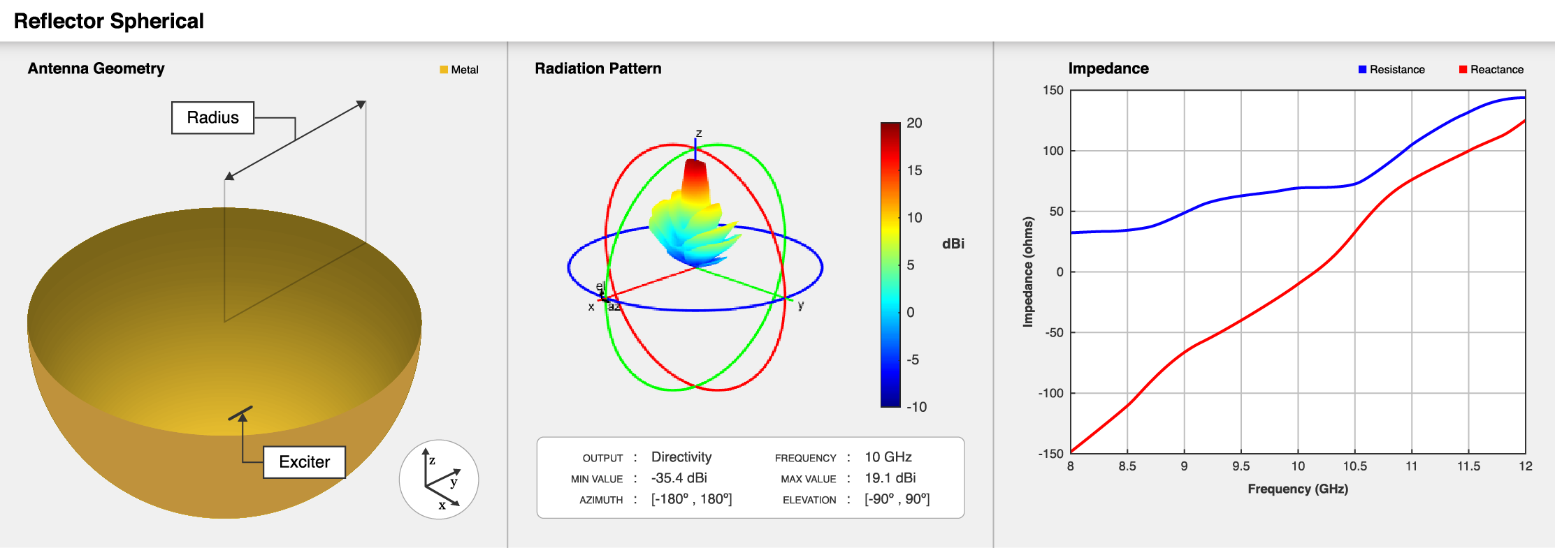
The reflectorSpherical antenna object creates a spherical reflector-backed antenna. The reflector in the spherical reflector-backed antenna is one-half the size of the sphere. The antenna is used in wide-angle scanning on account of its perfectly symmetrical geometric configuration.

Creation

Syntax

ant = reflectorSpherical

ant = reflectorSpherical(Name=Value)

Description

ant = reflectorSpherical creates a spherical reflector-backed antenna. The default antenna object has an exciter as a center-fed dipole located on the X-Y plane. The default antenna object dimensions are chosen for an operating frequency of 1 GHz.

ant = reflectorSpherical(Name=Value) creates a cavity-backed antenna, with additional Properties specified by one or more name–value arguments. Name is the property name and Value is the corresponding value. You can specify several name-value arguments in any order as Name1= Value1, ..., NameN=ValueN. Properties not specified retain their default values.

For example, reflectorSpherical(Radius=0.6) sets the spherical reflector radius to 0.6 meters.

Properties

Exciter — Antenna or array used as exciter

dipole (default) | antenna object | array object | custom antenna object | measuredAntenna object | empty array

Exciter antenna or array type, specified as either:

• Antenna object from the catalog (except reflector type, cavity type and platform-installed antennas)

• Array object from the catalog (except conformal and infinite arrays)

• Custom antennas: customAntennaGeometry, customAntennaMesh, customAntenna

• Measured pattern data of an antenna or array: measuredAntenna

• Empty array

To create the reflector backing structure without an exciter, specify this property as an empty array.

Example: dipole

Example: linearArray(Element=patchMicrostrip)

Example: customAntenna

Example: measuredAntenna

Example: []

Radius — Radius of spherical aperture

0.15 (default) | positive scalar

Aperture radius of the spherical reflector along X and Y-axes, specified as a positive scalar in meters.

Example: 0.259

Data Types: double

FeedOffset — Signed distance between feed point and origin

[0 0 0.075] (default) | three-element vector

Signed distance between feed point of the exciter and the origin, specified as a three-element vector with each element unit in meters.

Example: [0 0 0.082]

Data Types: double

Depth — Perpendicular distance between origin and aperture of antenna

0.15 (default) | positive scalar

Perpendicular distance between origin and the aperture of the spherical reflector-backed antenna, specified as a positive scalar in meters.

Example: 0.6

Note

Depth should be less than or half the Radius.

Data Types: double

Conductor — Type of metal material

"PEC" (default) | metal object

Type of the metal used as a conductor, specified as a metal material object. You can choose any metal from the MetalCatalog or specify a metal of your choice. For more information, see metal. For more information on metal conductor meshing, see Meshing.

Example: metal("Copper")

Tilt — Tilt angle of antenna

0 (default) | scalar | vector

Tilt angle of the antenna in degrees, specified as a scalar or vector. For more information, see Rotate Antennas and Arrays.

Example: 90

Example: Tilt=[90 90],TiltAxis=[0 1 0;0 1 1] tilts the antenna at 90 degrees about the two axes defined by the vectors.

Data Types: double

TiltAxis — Tilt axis of antenna

[1 0 0] (default) | three-element vector | 2-by-3 matrix | "X" | "Y" | "Z"

Tilt axis of the antenna, specified as one of these values:

• Three-element vector of Cartesian coordinates in meters. In this case, each coordinate in the vector starts at the origin and lies along the specified points on the x-, y-, and z-axes.

• Two points in space, specified as a 2-by-3 matrix corresponding to two three-element vectors of Cartesian coordinates. In this case, the antenna rotates around the line joining the two points.

• "x", "y", or "z" to describe a rotation about the x-, y-, or z-axis, respectively.

For more information, see Rotate Antennas and Arrays.

Example: [0 1 0]

Example: [0 0 0;0 1 0]

Example: "Z"

Data Types: double | string

Load — Lumped elements

[1x1 lumpedElement] (default) | lumpedElement object

Lumped elements added to the antenna feed, specified as a lumpedElement object. You can add a load anywhere on the surface of the antenna. By default, the load is at the feed. For more information, see lumpedElement.

Example: Load=lumpedelements, where lumpedelements is the load added to the antenna feed.

Example: lumpedElement(Impedance=75)

SolverType — Solver for antenna analysis

"MoM-PO" (default) | "MoM" | "PO" | "FMM"

Solver for antenna analysis, specified as a string. Default solver is "MoM-PO"(Method of Moments-Physical Optics hybrid). Other supported solvers are: "MoM" (Method of Moments), "PO" (Physical optics) or "FMM" (Fast Multipole Method).

Example: SolverType="MoM"

Data Types: string

Object Functions

axialRatio	Calculate and/or plot axial ratio of antenna or array
bandwidth	Calculate and/or plot absolute bandwidth of antenna
beamwidth	Beamwidth of antenna
current	Current distribution on antenna or array surface
charge	Charge distribution on antenna or array surface
design	Design prototype antenna or arrays for resonance around specified frequency or create AI-based antenna from antenna catalog objects
efficiency	Radiation efficiency of antenna
EHfields	Electric and magnetic fields of antennas or embedded electric and magnetic fields of antenna element in arrays
impedance	Input impedance of antenna or scan impedance of array
info	Display information about antenna, array, or platform
memoryEstimate	Estimate memory required to solve antenna or array mesh
mesh	Mesh properties of metal, dielectric antenna, or array structure
meshconfig	Change meshing mode of antenna, array, custom antenna, custom array, or custom geometry
optimize	Optimize antenna or array using SADEA optimizer
pattern	Plot radiation pattern and phase of antenna or array or embedded pattern of antenna element in array
patternAzimuth	Azimuth plane radiation pattern of antenna or array
patternElevation	Elevation plane radiation pattern of antenna or array
rcs	Calculate and plot monostatic and bistatic radar cross section (RCS) of platform, antenna, or array
resonantFrequency	Calculate and/or plot resonant frequency of antenna
returnLoss	Return loss of antenna or scan return loss of array
show	Display antenna, array structures, shapes, or platform
solver	Access FMM solver for electromagnetic analysis
sparameters	Calculate S-parameters for antennas and antenna arrays
vswr	Voltage standing wave ratio (VSWR) of antenna or array element

Examples

Design Spherical Reflector-Backed Antenna with Default Properties

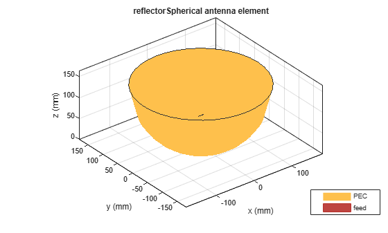
Create a spherical reflector-backed antenna object with default properties.

ant = reflectorSpherical

ant = 
  reflectorSpherical with properties:

       Exciter: [1x1 dipole]
        Radius: 0.1500
         Depth: 0.1500
    FeedOffset: [0 0 0.0750]
          Tilt: 0
      TiltAxis: [1 0 0]
          Load: [1x1 lumpedElement]
    SolverType: 'MoM-PO'

View the antenna.

show(ant)

Plot S-Parameter of Spherical Reflector-Backed Dipole Antenna

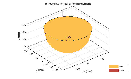
Create a spherical reflector-backed antenna with a dipole as an exciter spaced at 90 millimeters.

rs = reflectorSpherical;
rs.FeedOffset(3) = 90e-3;

Visualize the antenna.

figure
show(rs)

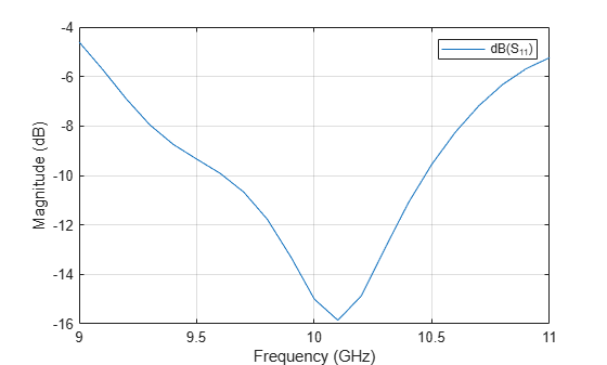
Plot the S-parameters at 1 GHz.

s = sparameters(rs,(9:0.1:11)*1e9);
figure
rfplot(s)

Plot Radiation Pattern of Spherical Reflector-Backed Waveguide Antenna

Create a waveguide designed at 10 GHz backed with a spherical reflector.

w = design(waveguide,10e9);
rs = reflectorSpherical(Exciter=w);
rs.Exciter.Tilt = 90;
rs.Exciter.TiltAxis = [ 0 1 0];

Visualize the antenna.

figure
show(rs)

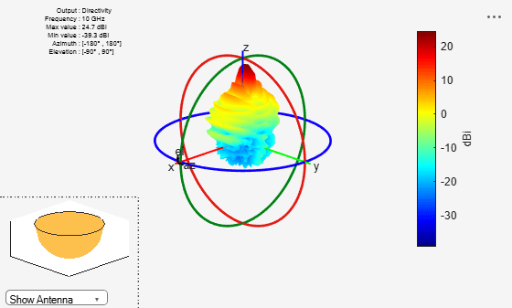
Plot the radiation pattern at 10 GHz.

figure
pattern(rs,10e9)

Create Spherical Reflector Antenna with Circular Array of Discone Antennas

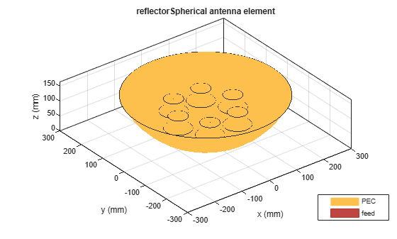
Create a circular array with discone antennas.

d = discone(Height=0.04);
circArr = circularArray(Element=d,Radius=0.1);

Create a spherical reflector antenna with circular array exciter.

ant = reflectorSpherical(Exciter=circArr,Radius=0.25)

ant = 
  reflectorSpherical with properties:

       Exciter: [1x1 circularArray]
        Radius: 0.2500
         Depth: 0.1500
    FeedOffset: [0 0 0.0750]
          Tilt: 0
      TiltAxis: [1 0 0]
          Load: [1x1 lumpedElement]
    SolverType: 'MoM-PO'

show(ant)

References

[1] Balanis, Constantine A. Antenna Theory: Analysis and Design. 3rd ed. Hoboken, NJ: John Wiley, 2005.

Version History

Introduced in R2020b