Main Content

sweeptone

R2026b

Exponential swept sine

The sweeptone function has changed. For more information, see Version History.

Description

excitation = sweeptone() returns an excitation signal generated using the Exponential Swept Sine (ESS) technique. By default, the signal has a 6.157-second duration, followed by 4 seconds of silence, for a sample rate of 44.1 kHz.

example

excitation = sweeptone(swDur) specifies the target duration of the ESS signal.

excitation = sweeptone(swDur,silDur) also specifies the duration of the silence following the ESS signal.

excitation = sweeptone(swDur,silDur,fs) also specifies the sample rate of the sweep tone as fs in Hz.

example

excitation = sweeptone(___,Name=Value) specifies additional options using one or more name-value arguments for any of the previous syntaxes. Options include the excitation level and the range of sweep frequency.

example

Examples

collapse all

Since R2026b

Generate a 6.157-second exponential swept sine (ESS) signal at a rate of 44.1 kHz. The sweep goes from 10 Hz to 22 kHz, followed by with a 4-second silence.

exc = sweeptone();

Visualize the excitation in time. The excitation level of –6 dB yields an amplitude of 10-6/20=0.5012V.

t = (0:numel(exc)-1)/44100;
plot(t,exc)
xlabel("Time (s)")
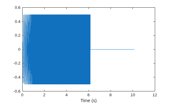
Figure contains an axes object. The axes object with xlabel Time (s) contains an object of type line.

Generate an exponential swept sine (ESS) signal sampled at a rate of 48 kHz. The sweep lasts for approximately 3 seconds and follows with a 2-second silence.

fs = 48e3;
exc = sweeptone(3,2,fs);

Visualize the excitation in the time-frequency domain. The default frequency sweep goes from 10 Hz to 22 kHz.

spectrogram(exc,512,0,1024,fs,"yaxis")
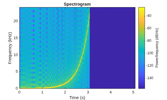
Figure contains an axes object. The axes object with title Spectrogram, xlabel Time (s), ylabel Frequency (kHz) contains an object of type image.

Create a sweep tone excitation signal with a sweep that goes from 20 Hz to 20 kHz for approximately 2 seconds and ends with a 1-second silence. Specify the sample rate as 44.1 kHz.

exc = sweeptone(2,1,44100,SweepFrequencyRange=[20 20e3]);

plot((0:numel(exc)-1)/44100,exc)
title("Excitation")
xlabel("Time (seconds)")
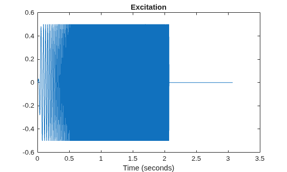
Figure contains an axes object. The axes object with title Excitation, xlabel Time (seconds) contains an object of type line.

Pass the excitation signal through an infinite impulse response (IIR) filter and add noise to model a real-world recording (system response).

[B,A] = butter(10,[0.1 0.7],"ctf");
rec = ctffilt(B,A,exc);
nrec = rec + 0.12*randn(size(rec));

plot((0:numel(nrec)-1)/44100,nrec)
title("System Response")
xlabel("Time (seconds)")
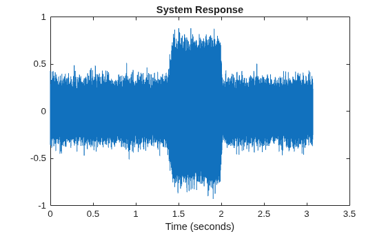
Figure contains an axes object. The axes object with title System Response, xlabel Time (seconds) contains an object of type line.

Pass the excitation signal and the system response to the impzest function to estimate the impulse response. Truncate the estimate to 100 points. Use impz to determine the true impulse response of the system. Plot the true impulse response and the estimated impulse response for comparison.

irEstimate = impzest(exc,nrec);
irEstimate = irEstimate(1:101);

irTrue = impz(B,A,101);
plot(0:100,irEstimate,"-",0:100,irTrue,"--")

legend(["True" "Estimated"] + " impulse response")
xlabel("Sample Number")
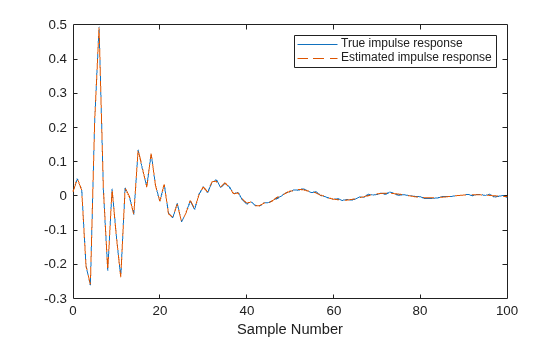
Figure contains an axes object. The axes object with xlabel Sample Number contains 2 objects of type line. These objects represent True impulse response, Estimated impulse response.

Input Arguments

collapse all

Target duration of the ESS signal (in seconds), specified as a scalar in the range [0.5, 60].

The actual duration, T, depends on swDur, the sample rate fs, and the range of sweep frequency specified as SweepFrequencyRange = [f1 f2]. The function adjusts the duration to ensure a synchronized phase of 0 radians at both ends of the ESS signal. This code calculates T:

T =  round(swDur*f1/log(f2/f1))/(f1/log(f2/f1))

The maximum difference between T and swDur is 0.5/(f1/log(f2/f1)) seconds.

Data Types: single | double

Duration of silence after ESS (in seconds), specified as a positive scalar.

Sample rate (in Hz), specified as a positive scalar.

Name-Value Arguments

collapse all

Specify optional pairs of arguments as Name1=Value1,...,NameN=ValueN, where Name is the argument name and Value is the corresponding value. Name-value arguments must appear after other arguments, but the order of the pairs does not matter.

Example: sweeptone(3,2,48e3,ExcitationLevel=-5)

Level of the excitation signal to generate (in dB), specified as a scalar in the range [–42, 0].

When you specify ExcitationLevel=a, the function scales the ESS signal by 10^(a/20) before returning excitation.

Data Types: single | double | int8 | int16 | int32 | int64 | uint8 | uint16 | uint32 | uint64

Range of sweep frequency in Hz, specified as a two-element positive-valued row vector. Each value must be unique.

  • You can specify the sweep frequency range as low to high or high to low. For example, [10 22000] and [22000 10] are both valid inputs.

  • The largest value of the sweep frequency range must be less than or equal to fs/2.

Data Types: single | double | int8 | int16 | int32 | int64 | uint8 | uint16 | uint32 | uint64

Output Arguments

collapse all

Excitation signal generated using the ESS technique, returned as a column vector. The length of the column vector is about (swDur+silDur)*fs samples.

Data Types: single | double

More About

collapse all

References

[1] Farina, A. "Advancements in Impulse Response Measurements by Sine Sweeps." Presented at the Audio Engineering Society 122nd Convention, Vienna, Austria, 2007.

[2] Novák, A., Simon, L, Kadlec, F., and Lotton, P. "Nonlinear System Identification Using Exponential Swept-Sine Signal." IEEE Transactions on Instrumentation and Measurement, Vol. 59, No. 8, pp. 2220-2229, 2009.

Extended Capabilities

expand all

C/C++ Code Generation
Generate C and C++ code using MATLAB® Coder™.

Version History

Introduced in R2018b

expand all