siteviewer
Create Site Viewer
Description
Display transmitter sites, receiver sites, and RF propagation visualizations
by using a siteviewer object.
Site Viewer has two visualization modes:
3-D globe — Display sites that are referenced to geographic coordinates. You can customize the globe using custom terrain, high-zoom-level or custom basemaps, and buildings. This is the default visualization mode.
3-D model — Display sites that are referenced to Cartesian coordinates. You can import and view 3-D models represented by glTF™ files (since R2023b), standard tessellation language (STL) files, or
triangulationobjects. Specify the 3-D model by using theSceneModelname-value argument.
Site Viewer requires hardware graphics support for WebGL™.
Creation
Description
viewer = siteviewer
viewer = siteviewer(PropertyName=Value)CoordinateSystem and Materials.
For example, you can import and view a 3-D model file by using the SceneModel name-value argument.
Properties
Site Viewer
Caption to display on map viewer window, specified as a character vector or a string scalar.
Data Types: char | string
Size and location of map viewer window in pixels, specified as a
four-element integer-valued vector in the form [left bottom
width height]. The default value depends on the screen
resolution such that the window lies in the center of the screen with a
width of 800 pixels and a height of 600 pixels.
Data Types: double
This property is read-only.
Coordinate reference system, specified as
"geographic" or "cartesian".
The value of CoordinateSystem depends on how you
create the Site Viewer.
By default, the value of
CoordinateSystemis"geographic"and visualizations are referenced to the WGS84 reference ellipsoid.When you create the Site Viewer by specifying the
SceneModelargument, the value ofCoordinateSystemis"cartesian"and the coordinates are defined by the origin of the 3-D model.
When CoordinateSystem is
"geographic", you can view the latitude and
longitude coordinates for a location by right-clicking the map and
selecting Show Location. To remove the location,
right-click and select Remove Location.
Data Types: char | string
Since R2023b
This property is read-only.
Scene materials, returned as a table. When you create a scene from a
glTF file, an OpenStreetMap® file, or a geospatial table, Site Viewer assigns materials
to the surfaces in the scene by matching each material name stored in
the file or table with the name of a supported material. By default,
when you perform ray tracing analysis by using a function such as
raytrace or coverage, the function uses the matched material
names.
For each material stored in the file or geospatial table, the scene materials table contains these variables:
Material— Name of the material stored in the file or geospatial table, returned as a string scalar.MatchedCatalogMaterial— Name of the matched material, returned as one of these values:""— Material is not supported. By default, the ray tracing analysis functions use concrete for materials that are not supported.A material name from this table.
Common Building Materials Metals Terrestrial Materials Theoretical Materials "acrylic"— Acrylic"brick"— Brick"ceiling-board"— Ceiling board"chipboard"— Chipboard"concrete"— Concrete"floorboard"— Floorboard"foam"— Foam"FR4"— FR-4 (fiberglass)"glass"— Glass"marble"— Marble"metal"— Metal"plasterboard"— Plasterboard"plywood"— Plywood"polystyrene"— Polystyrene"Teflon"— Teflon® (PTFE)"wood"— Wood
"aluminum"— Aluminum"brass"— Brass"copper"— Copper"gold"— Gold"Invar"— Invar"iron"— Iron"lead"— Lead"silver"— Silver"steel"— Steel"tungsten"— Tungsten"zinc"— Zinc
"air"— Air"ice"— Ice"loam"— Loam"seawater"— Seawater"snow"— Snow"tree"— Tree"vegetation"— Vegetation"water"— Water
"PEC"— Perfect electrical conductor"vacuum"— Vacuum (free space)
Ray tracing models calculate propagation loss using the electromagnetic properties of the scene materials. For more information about the electromagnetic properties used by ray tracing models, see Properties of Ray Tracing Materials.
Data Types: table
Geographic Coordinate System
Map imagery used to visualize sites, specified as one of the basemap
names in this table or as a custom basemap defined using the addCustomBasemap function.
|
|
Full global basemap composed of high-resolution satellite imagery. Hosted by Esri®. |
|
Street map provided by OpenStreetMap. |
|
|
General-purpose road map that emphasizes accurate, legible styling of roads and transit networks. Hosted by Esri. |
|
Map designed to provide geographic context while highlighting user data on a light background. Hosted by Esri. |
|
|
Map designed to provide geographic context while highlighting user data on a dark background. Hosted by Esri. |
|
General-purpose map with styling to depict topographic features. Hosted by Esri. |
|
|
Map that combines satellite-derived land cover data, shaded relief, and ocean-bottom relief. The light, natural palette is suitable for thematic and reference maps. Created using Natural Earth. |
|
Shaded relief map blended with a land cover palette. Humid lowlands are green and arid lowlands are brown. Created using Natural Earth. |
|
|
Terrain map in shades of gray. Shaded relief emphasizes both high mountains and micro-terrain found in lowlands. Created using Natural Earth. |
|
Two-tone, land-ocean map with light green land areas and light blue water areas. Created using Natural Earth. |
|
|
Two-tone, land-ocean map with gray land areas and white water areas. Created using Natural Earth. |
|
Two-tone, land-ocean map with light gray land areas and dark gray water areas. This basemap is installed with MATLAB®. Created using Natural Earth. |


The basemaps hosted by Esri update periodically. As a result, you might see differences in your visualizations over time.
Alignment of boundaries and region labels are a presentation of the feature provided by the data vendors and do not imply endorsement by MathWorks®.
This property applies only when CoordinateSystem
is "geographic".
Data Types: char | string
Data on which to visualize sites and perform terrain calculations,
specified as a character vector or a scalar previously added using
addCustomTerrain or one of the following options:
'none'— Terrain elevation is0everywhere.'gmted2010'— USGS GMTED2010 terrain data. This option requires an internet connection.
This property applies only when CoordinateSystem
is "geographic".
This property is read-only after you create the Site Viewer.
For limitations, see Limitations.
Data Types: char | string
Buildings data, specified as one of these options:
A string scalar or character vector that specifies the name of an OpenStreetMap file (
.osm).A geospatial table. A geospatial table is a
tableortimetablewith aShapetable variable and attribute table variables. TheShapetable variable must containgeopolyshape(Mapping Toolbox) objects. This option requires Mapping Toolbox™.
If you specify the name of an OpenStreetMap file, the way you specify the file depends on the location of the file.
If the file is in your current folder or in a folder on the MATLAB path, then specify the name of the file, such as
"myFile.osm".If the file is not in the current folder or in a folder on the MATLAB path, then specify the full or relative path name, such as
"C:\myfolder\myFile.osm"or"dataDir\myFile.osm".
This property applies only when the
CoordinateSystem property is set to
"geographic".
This property is read-only after you create the Site Viewer.
For limitations, see Limitations.
Data Types: char | string | table
Cartesian Coordinate System
Name
of the 3-D model file or 3-D triangulation data, specified as a string
scalar, a character vector, a triangulation object, or
"none".
Specify the name of a 3-D model file using a string scalar or a character vector. Site Viewer supports these 3-D model file formats:
glTF (
.gltf,.glb) (since R2023b)STL (
.stl)
The way you specify the file depends on the location of the file.
If the file is in your current folder or in a folder on the MATLAB path, then specify the name of the file, such as
"myFile.stl".If the file is not in the current folder or in a folder on the MATLAB path, then specify the full or relative path name, such as
"C:\myfolder\myFile.stl"or"dataDir\myFile.stl".
Specify 3-D triangulation data using a
triangulationobject.Specify no 3-D model using
"none".
This property applies only when the
CoordinateSystem property is set to
"cartesian".
This property is read-only after you create the Site Viewer.
Since R2023b
Scale of the 3-D model, specified as a positive scalar. When you
import a 3-D model from a glTF file, an STL file, or a triangulation
object, Site Viewer creates the scene by multiplying this value by the
linear distances stored in the model. For example, when the distance
between two vertices in the model is 10 units, specifying this value as
2 increases the distance to 20 units.
By default, Site Viewer interprets scene models using units of meters with a 1:1 scale.
This property applies only when the
CoordinateSystem property is set to
"cartesian".
This property is read-only after you create the Site Viewer.
Transparency of the model, specified as a scalar in the range
[0,1], where 0 is transparent
and 1 is opaque.
The default value depends on the values of the
ShowEdges and SceneModel properties.
When
ShowEdgesis1(true), the default value is0.1. WhenShowEdgesis0(false), the default value is1.When
SceneModelcontains the name of a glTF file, the default is1.
This property applies only when the
CoordinateSystem property is set to
"cartesian".
Data Types: double
Option to show the origin of the model, specified as
"on" or "off", or as numeric
or logical 1 (true) or
0 (false). A value of
"on" is equivalent to true,
and "off" is equivalent to false.
Thus, you can use the value of this property as a logical value. The
value is stored as an on/off logical value of type matlab.lang.OnOffSwitchState.
The x-axis appears in red, the y-axis appears in green, and the z-axis appears in blue. The z-axis of the scene points up.
This property applies only when the
CoordinateSystem property is set to
"cartesian".
Option to show the edges of the model using black lines, specified as
"on" or "off", or as numeric
or logical 1 (true) or
0 (false). A value of
"on" is equivalent to true,
and "off" is equivalent to false.
Thus, you can use the value of this property as a logical value. The
value is stored as an on/off logical value of type matlab.lang.OnOffSwitchState.
Site Viewer defines edges as two adjacent facets with normals that differ by more than 2 degrees.
This property applies only when the
CoordinateSystem property is set to
"cartesian".
This property is read-only after you create the Site Viewer.
Object Functions
campos | Set or query position of camera for Site Viewer |
camheight | Set or query height of camera for Site Viewer |
camheading | Set or query heading angle of camera for Site Viewer |
campitch | Set or query pitch angle of camera for Site Viewer |
camroll | Set or query roll angle of camera for Site Viewer |
clearMap | Clear plots |
close | Close Site Viewer |
Examples
Create a default Site Viewer.
viewer = siteviewer;

Pan by left-clicking and dragging, zoom by right-clicking and dragging or by using the scroll wheel, and rotate the visualization by clicking the middle button and dragging or by pressing Ctrl and left-clicking or dragging. View the coordinates for a location by right-clicking and selecting Show location.
For this example, navigate to a region containing New England and view the coordinates for a location near Cape Cod.

A gray marker appears at the location you selected. Remove the marker by right-clicking the location and selecting Remove location.
Since R2023b
View a 3-D model from a glTF file created using RoadRunner. RoadRunner is an interactive editor that lets you design 3-D scenes for simulating and testing automated driving systems.
Create a temporary folder to store a sample glTF file. Download the file into the folder by using the downloadGLTFFile helper function. The helper function is attached to the example as a supporting file.
dataDir = fullfile(tempdir,"IntersectionAndBuildings");
if ~exist(dataDir,"dir")
    mkdir(dataDir)
end
downloadGLTFFile(dataDir)
The glTF file consists of one main file that defines the structure of the model and multiple image files that define the colors and textures of the model. Specify the name of the main file. Then, import and view the glTF file using Site Viewer.
filename = fullfile(dataDir,"IntersectionAndBuildings.glb");
viewer = siteviewer(SceneModel=filename,ShowEdges=false,ShowOrigin=false);
Site Viewer displays the model using the colors and textures stored with the file. Adjust the view by changing the camera position and the camera rotation angles. Specify the position using meters and the rotation angles using degrees.
campos(viewer,-26,-57,37)
campitch(viewer,-25)
camheading(viewer,-26)

Import and view an STL file. The file models a small conference room with one table and four chairs.
viewer = siteviewer(SceneModel="conferenceroom.stl");Pan by left-clicking, zoom by right-clicking or by using the scroll wheel, and rotate the visualization by clicking the middle button and dragging or by pressing Ctrl and left-clicking and dragging.

Launch Site Viewer with a basemap and buildings file for Manhattan. Site Viewer displays the buildings using the colors stored in the file. For more information about the OpenStreetMap® file, see [1].
viewer = siteviewer(Basemap="openstreetmap",Buildings="manhattan.osm");

Show a transmitter site on a building.
tx = txsite(Latitude=40.7107,Longitude=-74.0114,AntennaHeight=50);
show(tx)

Appendix
[1] The OpenStreetMap file is downloaded from https://www.openstreetmap.org, which provides access to crowd-sourced map data all over the world. The data is licensed under the Open Data Commons Open Database License (ODbL), https://opendatacommons.org/licenses/odbl/.
Customize the buildings stored in an OpenStreetMap® file by reading the buildings into a geospatial table, editing the geospatial table, and importing the geospatial table into Site Viewer.
Read building parts from an OpenStreetMap file [1] by using the readgeotable (Mapping Toolbox) function. The function derives information about the buildings from the file and stores the result in a geospatial table. The Shape table variable represents the buildings using polygon shapes in geographic coordinates.
buildings = readgeotable("manhattan.osm",Layer="buildingparts");
buildings.Shape
ans=2821×1 geopolyshape array with properties:
              NumRegions: [2821×1 double]
                NumHoles: [2821×1 double]
                Geometry: "polygon"
    CoordinateSystemType: "geographic"
           GeographicCRS: [1×1 geocrs]
      ⋮
Find the unique building materials reported by the OpenStreetMap file.
uniqueMaterials = unique(buildings.Material)
uniqueMaterials = 8×1 string
    ""
    "brick"
    "concrete"
    "copper"
    "glass"
    "metal"
    "plaster"
    "stone"
Create a dictionary that associates each material with a color. Specify the colors using hexadecimal color codes. Use gray for unspecified materials and concrete, red for brick, orange for copper, blue for glass, black for metal, white for plaster, and purple for stone.
materials = ["","brick","concrete","copper","glass","metal","plaster","stone"];
colors = ["#D3D3D3","#AA4A44","#D3D3D3","#B87333","#35707E","#151513","#FFFFFF","#301934"];
dict = dictionary(materials,colors)
dict =

  dictionary (string ⟼ string) with 8 entries:

    ""         ⟼ "#D3D3D3"
    "brick"    ⟼ "#AA4A44"
    "concrete" ⟼ "#D3D3D3"
    "copper"   ⟼ "#B87333"
    "glass"    ⟼ "#35707E"
    "metal"    ⟼ "#151513"
    "plaster"  ⟼ "#FFFFFF"
    "stone"    ⟼ "#301934"
For each building in the table, set the color of the building based on the building material.
numBuildings = height(buildings);
for n = 1:numBuildings
    material = buildings.Material(n);
    buildings.Color(n) = dict(material);
end
Display the buildings in Site Viewer. Navigate to an area that shows several building colors.
viewer = siteviewer(Buildings=buildings);

View the building materials stored in the Site Viewer by querying the Materials property of the Site Viewer object. By default, ray tracing analysis functions use the materials stored in the MatchedCatalogMaterial table variable.
viewer.Materials
ans=7×2 table
     Material     MatchedCatalogMaterial
    __________    ______________________

    "brick"           "brick"
    "concrete"        "concrete"
    "copper"          "copper"
    "glass"           "glass"
    "metal"           "metal"
    "plaster"         "plasterboard"
    "stone"           "marble"
[1] The OpenStreetMap file is downloaded from https://www.openstreetmap.org, which provides access to crowd-sourced map data all over the world. The data is licensed under the Open Data Commons Open Database License (ODbL), https://opendatacommons.org/licenses/odbl/.
Add a custom basemap to view locations on an OpenTopoMap® basemap, then remove the custom basemap.
Specify values for these arguments:
A name that identifies the custom basemap.
The URL of the map tiles. For load balancing, this provider has three servers that you can use (
a,b, orc).An attribution that gives credit to the provider of the map tiles. When you plot data, this attribution appears at the bottom of the map. Map tile providers can define specific requirements for the attribution.
A display name for the custom basemap. This name appears in the Imagery tab of Site Viewer.
name = "opentopomap";
url = "a.tile.opentopomap.org/${z}/${x}/${y}.png";
attribution = "©OpenStreetMap contributors";
displayName = "Open Topo Map";
Use addCustomBasemap to load the custom basemap, and then create a Site Viewer that uses the custom basemap.
addCustomBasemap(name,url,Attribution=attribution,DisplayName=displayName)
viewer = siteviewer(Basemap=name);
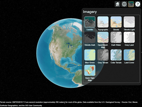
After you add a custom basemap, the custom map is available in new Site Viewer windows. Note the Open Topo Map basemap icon in the Imagery tab.
viewer2 = siteviewer;
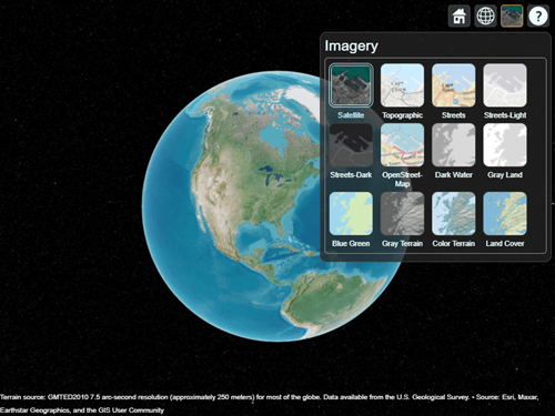
Use removeCustomBasemap to remove the custom basemap. Then, open a new Site Viewer. Note the Open Topo Map basemap option is no longer available in the Imagery tab.
removeCustomBasemap(name)
viewer3 = siteviewer;
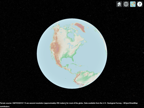
Launch two Site Viewer windows: one that uses terrain data derived from the GMTED2010 model by the USGS and NGA, and one without terrain data.
viewer1 = siteviewer(Terrain="gmted2010",Name="Site Viewer (GMTED2010)");
viewer2 = siteviewer(Terrain="none",Name="Site Viewer (No Terrain Data)");
Create a transmitter site.
tx = txsite;
Generate a coverage map on each window. The map with terrain uses the Longley-Rice propagation model by default.
coverage(tx,Map=viewer1)

The map without terrain uses the free-space model by default.
coverage(tx,Map=viewer2)

Limitations
Terrain
Default terrain access requires an internet connection. If no internet connection exists, then Site Viewer automatically uses
'none'in the propertyTerrain.Custom DTED terrain files for use with
addCustomTerrainmust be acquired outside of MATLAB for example by using USGS EarthExplorer.When using custom terrain, analysis is restricted to the terrain region. For example, an error occurs if you are trying to show a transmitter or receiver site outside of the region.
Buildings
OpenStreetMap files obtained from https://www.openstreetmap.org represent crowd-sourced map data, and the completeness and accuracy of the buildings data may vary depending on the map location.
When downloading data from https://www.openstreetmap.org, select an export area larger than the desired area to ensure that all expected building features are fully captured. Building features at the edge of the selected export area may be missing.
Building geometry and features are interpreted from the file according to the recommendations of OpenStreetMap for 3-D buildings.
MATLAB Online
In MATLAB Online™, if you refresh the URL, then the Site Viewer window remains open but the visualizations disappear.
More About
You can interactively navigate Site Viewer by using your mouse.
Pan by left-clicking and dragging.
Zoom by scrolling or by right-clicking and dragging.
Tilt and rotate by holding Ctrl and dragging or by middle-clicking and dragging.
When CoordinateSystem is "geographic", you
can restore the default view by selecting ![]() Restore View from the toolbar.
Restore View from the toolbar.
To programmatically navigate Site Viewer, use the campos,
camheight,
camheading,
campitch, and
camroll
functions.
When CoordinateSystem is
"geographic", you can choose between three view options by
using the Dimension Picker in the toolbar.
 3-D View — A smooth globe. This is the default
view.
3-D View — A smooth globe. This is the default
view. 2-D View — A flat map in the Mercator
projection.
2-D View — A flat map in the Mercator
projection. Columbus View — A flat map in the Mercator
projection that supports tilt and rotation.
Columbus View — A flat map in the Mercator
projection that supports tilt and rotation.
Some interactions are not supported for 2-D View and Columbus View.
Version History
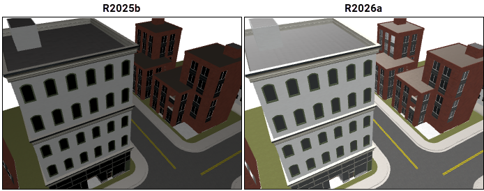
Introduced in R2019bWhen you read a scene model from a glTF file into Site Viewer, the model has a brighter appearance. This figure compares a scene model in Site Viewer in R2025b and R2026a.