Structurally Compress Neural Network DPD Using Projection

Since R2024a

This example uses:

Step 4 of 6 in AI for Digital Predistortion Design

This example shows how to structurally compress a neural network digital predisposition design (NN-DPD) to reduce computational complexity and memory requirements by using projection and principal component analysis.

Introduction

There are two primary neural network compression techniques. Specifically, structural compression by pruning or projection, and data type compression by quantization. This example focuses on structural compression through projection. To structurally compress a deep learning network, you can use projected layers. The layer introduces learnable projector matrix $Q$ , replaces multiplications of the form $W x$ (where $W$ is a learnable matrix) with the multiplication $W Q Q^{⊤} x$ , and stores $Q$ and $W' = W Q$ (instead of storing $W$ ). In some cases, this is equivalent to replacing a layer with a subnetwork of smaller layers. Projecting $x$ into a lower dimensional space using $Q$ typically requires less memory to store the learnable parameters and can have similarly strong prediction accuracy. A projected deep neural network can also exhibit faster forward passes when run on the CPU or deployed to embedded hardware using library-free C or C++ code generation.

The compressNetworkUsingProjection function compresses a network by projecting layers into smaller parameter subspaces. For optimal initialization of the projected network, the function projects the learnable parameters of projectable layers into a subspace that maintains the highest variance in neuron activations. After you compress a neural network using projection, fine-tune the network to increase the accuracy. For more information, see the Compress Neural Network Using Projection (Deep Learning Toolbox) example.

Sections of this example step through this workflow to compress a NN-DPD.

Load a pretrained network.
Compress using projection to obtain projected neural network.
Fine-tune projected neural network.
Test the NMSE performance and compare complexity to the original one.

Prepare Data and Neural Network

The following summarizes the data generation process and loads a pretrained network. For more information on data generation, see the Data Preparation for Neural Network Digital Predistortion Design example. For more information on design and training a neural network DPD, see the Neural Network for Digital Predistortion Design-Offline Training example.

Choose Data Source

Choose the data source for the power amplifier (PA) output. This example uses an NXP™ Airfast LDMOS Doherty PA, which is connected to a local NI™ VST, as described in the Power Amplifier Characterization example. If you do not have access to a PA, run the example with simulated PA or saved data. Simulated PA uses a neural network PA model, which is trained using data captured from the PA using an NI VST. If you choose saved data, the example downloads the data files.

dataSource = "Simulated PA";
if strcmp(dataSource,"Saved data")
  helperNNDPDDownloadData("projection")
end

Load Trained Neural Network

Load the trained neural network DPD together with memory depth and nonlinearity degree values used in the Neural Network for Digital Predistortion Design-Offline Training example.

load nndpdIn30Fact08 netDPD memDepth nonlinearDegree
netOriginal = netDPD

netOriginal = 
  dlnetwork with properties:

         Layers: [8x1 nnet.cnn.layer.Layer]
    Connections: [7x2 table]
     Learnables: [8x3 table]
          State: [0x3 table]
     InputNames: {'input'}
    OutputNames: {'linearOutput'}
    Initialized: 1

  View summary with summary.

figure
plot(netOriginal)

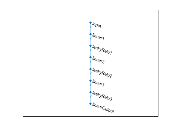
To display the network summary that shows whether the network is initialized, the total number of learnable parameters, and information about the network inputs, use the summary (Deep Learning Toolbox) function.

summary(netOriginal)

   Initialized: true

   Number of learnables: 2.1k

   Inputs:
      1   'input'   30 features

To display the number of nonzero learnable parameters (weights and biases), total number of multiplications and additions and memory required to store all of the learnable parameters for each layer in the network, use the estimateNetworkMetrics (Deep Learning Toolbox) function.

metricsOriginal = estimateNetworkMetrics(netOriginal);
metricsOriginal(:,[1 3 4 5])

ans=4×4 table
      LayerName       NumberOfLearnables    NumberOfOperations    ParameterMemory (MB)
    ______________    __________________    __________________    ____________________

    "linear1"                930                   1800                 0.0035477     
    "linear2"                744                   1440                 0.0028381     
    "linear3"                475                    912                  0.001812     
    "linearOutput"            40                     76                0.00015259

Generate Training Data

Generate training data as described in the Neural Network for Digital Predistortion Design-Offline Training example.

[txWaveTrain,txWaveVal,txWaveTest,ofdmParams] = generateOversampledOFDMSignals;

Pass signals through the PA.

pa = helperNNDPDPowerAmplifier(DataSource=dataSource, ...
  SampleRate=ofdmParams.SampleRate);
paOutputTrain = pa(txWaveTrain);
paOutputVal = pa(txWaveVal);
paOutputTest = pa(txWaveTest);

Preprocess the training data as described in the Neural Network for Digital Predistortion Design-Offline Training example. Create input preprocessing objects to generate input vectors containing features. During training and validation, use the PA output as NN-DPD input and the PA input as the NN-DPD output.

[inputMtxTrain,inputMtxVal,inputMtxTest,outputMtxTrain,outputMtxVal,outputMtxTest,scalingFactor] = ...
  helperNNDPDPreprocessData(txWaveTrain,txWaveVal,txWaveTest,paOutputTrain,paOutputVal,paOutputTest, ...
  memDepth,nonlinearDegree);

Analyze Neuron Activations for Compression Using Projection

The compressNetworkUsingProjection function uses principal component analysis (PCA) to identify the subspace of learnable parameters that result in the highest variance in neuron activations by analyzing the network activations using a data set of training data. This analysis requires only the predictors of the training data to compute the network activations. It does not require the training targets.

PCA can be computationally intensive. If you expect to compress the same network multiple times (for example, when exploring different levels of compression), then perform PCA first and reuse the resulting neuronPCA object.

Create the neuronPCA object. To view information about the steps of the neuron PCA algorithm, set the VerbosityLevel option to "steps".

dlXTest = dlarray(inputMtxTest,'BC');
npca = neuronPCA(netOriginal,dlXTest,VerbosityLevel="steps");

Using solver mode "direct".
Computing covariance matrices for activations connected to: "linear1/in","linear1/out","linear2/in","linear2/out","linear3/in","linear3/out","linearOutput/in","linearOutput/out"
Computing eigenvalues and eigenvectors for activations connected to: "linear1/in","linear1/out","linear2/in","linear2/out","linear3/in","linear3/out","linearOutput/in","linearOutput/out"
neuronPCA analyzed 4 layers: "linear1","linear2","linear3","linearOutput"

View the properties of the neuronPCA object.

npca

npca = 
  neuronPCA with properties:

                  LayerNames: ["linear1"    "linear2"    "linear3"    "linearOutput"]
      ExplainedVarianceRange: [0 1]
    LearnablesReductionRange: [0 0.8826]
            InputEigenvalues: {[30x1 double]  [30x1 double]  [24x1 double]  [19x1 double]}
           InputEigenvectors: {[30x30 double]  [30x30 double]  [24x24 double]  [19x19 double]}
           OutputEigenvalues: {[30x1 double]  [24x1 double]  [19x1 double]  [2x1 double]}
          OutputEigenvectors: {[30x30 double]  [24x24 double]  [19x19 double]  [2x2 double]}

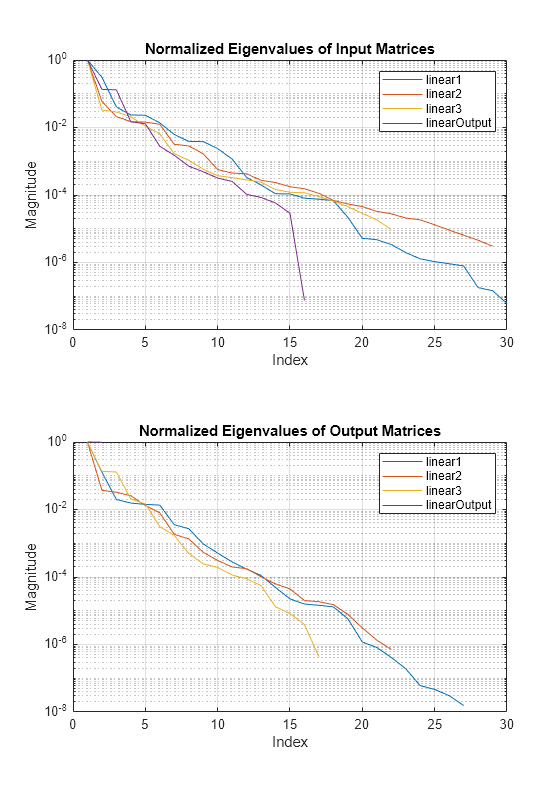
Plot the magnitude of the eigenvalues. Normalized eigenvalue magnitude (importance) drops significantly (below 1e-3) after 10-15th value, which shows that it might be possible to compress the neural network to 50% or more of its original size.

figure(Position=[0 0 560 800])
tiledlayout("vertical")
nexttile
semilogy(npca.InputEigenvalues{1}/max(npca.InputEigenvalues{1}))
hold on
semilogy(npca.InputEigenvalues{2}/max(npca.InputEigenvalues{2}))
semilogy(npca.InputEigenvalues{3}/max(npca.InputEigenvalues{3}))
semilogy(npca.InputEigenvalues{4}/max(npca.InputEigenvalues{4}))
hold off
grid on
title("Normalized Eigenvalues of Input Matrices")
xlabel("Index")
ylabel("Magnitude")
legend(npca.LayerNames)
nexttile
semilogy(npca.OutputEigenvalues{1}/max(npca.OutputEigenvalues{1}))
hold on
semilogy(npca.OutputEigenvalues{2}/max(npca.OutputEigenvalues{2}))
semilogy(npca.OutputEigenvalues{3}/max(npca.OutputEigenvalues{3}))
semilogy(npca.OutputEigenvalues{4}/max(npca.OutputEigenvalues{4}))
hold off
grid on
title("Normalized Eigenvalues of Output Matrices")
xlabel("Index")
ylabel("Magnitude")
legend(npca.LayerNames)

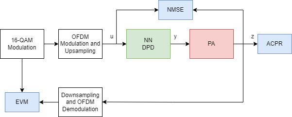
Test DPD Performance

This figure shows how to check the performance of the NN-DPD. To test the NN-DPD, pass the test signal through the NN-DPD and the PA and examine performance metrics such as normalized mean square error (NMSE), adjacent channel power ratio (ACPR), and error vector measurement (EVM). For more detail, see Neural Network for Digital Predistortion Design-Offline Training example. In this example, use the NMSE measured between the input to the NN-DPD and output of the PA.

NNDPD Offline test architecture

Pass the signal through original NN-DPD.

dpdOutNN = predict(netOriginal,inputMtxTest);
dpdOutNN = double(complex(dpdOutNN(:,1),dpdOutNN(:,2)));
dpdOutNN = dpdOutNN/scalingFactor;
paOutputNNOriginal = pa(dpdOutNN);

For comparison, the pass signal through the memory polynomial DPD.

estimator = comm.DPDCoefficientEstimator( ...
  'DesiredAmplitudeGaindB',0, ...
  'PolynomialType','Cross-term memory polynomial', ...
  'Degree',nonlinearDegree,'MemoryDepth',memDepth,'Algorithm','Least squares');
coef = estimator(txWaveTrain,paOutputTrain);

Warning: Rank deficient, rank = 16, tol =  1.107984e-03.

dpdMem = comm.DPD('PolynomialType','Cross-term memory polynomial', ...
  'Coefficients',coef);
dpdOutMP = dpdMem(txWaveTest);
paOutputMP = pa(dpdOutMP);

Calculate the NMSE of the original network using the test data. Record the values for further comparison.

nmseOriginal = helperNMSE(txWaveTest,paOutputNNOriginal)

nmseOriginal = single
    -33.4234

nmseMPDPD = helperNMSE(txWaveTest,paOutputMP)

nmseMPDPD = single
    -27.9844

Explore Compression Levels with Fine Tuning

There is a trade-off between the amount of compression and the network accuracy. Reducing the number of learnable parameters typically reduces the network accuracy.

To explore different amounts of compression, you can iterate over different values of the LearnablesReductionGoal option of the compressNetworkUsingProjection function and compare the results.

Loop over different values of the learnables reduction goal. Iterate over values between 20% and 80%. Any learnables reduction goal higher than 80% causes the output of the projected network to have too much distortion to be useful.

learnablesReductionGoal = 0.2:0.05:0.80;

For each value:

Compress the network using projection with the specified explained variance goal using the compressNetworkUsingProjection function. Suppress verbose output by setting the VerbosityLevel option to "off".
Record the actual explained variance and learnables reduction of the projected network.
Fine-tune the projected network. To reduce the training time, set maximum epochs to 50.
Calculate the NMSE of the projected network using the test data.

Specify the training options. Choosing among the options requires empirical analysis. Use Experiment Manager (Deep Learning Toolbox) to optimize hyperparameters.

maxEpochs = 50;
miniBatchSize = 512;
iterPerEpoch = floor(size(inputMtxTrain, 1)/miniBatchSize);
trainingPlots = "none";
metrics = [];
verbose = true;

options = trainingOptions('adam', ...
    MaxEpochs=maxEpochs, ...
    MiniBatchSize=miniBatchSize, ...
    InitialLearnRate=4e-4, ...
    LearnRateDropFactor=0.95, ...
    LearnRateDropPeriod=5, ...
    LearnRateSchedule='piecewise', ...
    Shuffle='every-epoch', ...
    OutputNetwork='best-validation-loss', ...
    ValidationData={inputMtxVal,outputMtxVal}, ...
    ValidationFrequency=10*iterPerEpoch, ...
    ValidationPatience=5, ...
    InputDataFormats="BC", ...
    TargetDataFormats="BC", ...
    ExecutionEnvironment='cpu', ...
    Plots=trainingPlots, ...
    Metrics = metrics, ...
    Verbose=verbose, ...
    VerboseFrequency=10*iterPerEpoch);

When running the example, you have the option of using a pretrained network by setting the trainNow variable to false. Training is desirable to match the network to your simulation configuration. If using a different PA, signal bandwidth, or target input power level, retrain the network. Training the neural network on an Intel® Xeon® W-2133 CPU takes about 6 minutes to satisfy the early stopping criteria specified above.

trainNow = false;

Compress, fine-tune, and measure the NMSE in a loop.

explainedVariance = zeros(size(learnablesReductionGoal));
learnablesReduction = zeros(size(learnablesReductionGoal));
nmseProjectedVec = zeros(size(learnablesReductionGoal));
nmseFineTunedVec = zeros(size(learnablesReductionGoal));
t = tic;
for p = 1:numel(learnablesReductionGoal)
    reductionGoal = learnablesReductionGoal(p);

    [netProjected,info] = compressNetworkUsingProjection(netOriginal,npca, ...
        LearnablesReductionGoal=reductionGoal, ...
        VerbosityLevel="off", ...
        LayerNames=["linear1","linear2","linear3"], ...
        UnpackProjectedLayers=true);

    explainedVariance(p) = info.ExplainedVariance;
    learnablesReduction(p) = info.LearnablesReduction;

    if trainNow
      netFineTuned = trainnet(inputMtxTrain,outputMtxTrain,netProjected,"mse",options);
    else
      load compressionLevelExplorationNetworks.mat netFineTunedVec
      netFineTuned = netFineTunedVec(p);
    end

    % Pass signal through projected NN-DPD
    dpdOutNN = predict(netProjected,inputMtxTest);
    dpdOutNN = double(complex(dpdOutNN(:,1),dpdOutNN(:,2)));
    dpdOutNN = dpdOutNN/scalingFactor;
    try 
      paOutputNNProjected = pa(dpdOutNN);
    catch
      paOutputNNProjected = nan(size(paOutputNNProjected));
    end

    % Pass signal through fine-tuned NN-DPD
    dpdOutNN = predict(netFineTuned,inputMtxTest);
    dpdOutNN = double(complex(dpdOutNN(:,1),dpdOutNN(:,2)));
    dpdOutNN = dpdOutNN/scalingFactor;
    paOutputNNFineTuned = pa(dpdOutNN);

    nmseProjectedVec(p) = helperNMSE(txWaveTest,paOutputNNProjected);
    nmseFineTunedVec(p) = helperNMSE(txWaveTest,paOutputNNFineTuned);
    fprintf("%s - %d%% reduction goal\n", ...
      duration(seconds(toc(t)),Format="hh:mm:ss"),round(reductionGoal*100))
end

00:00:03 - 20% reduction goal
00:00:07 - 25% reduction goal
00:00:10 - 30% reduction goal
00:00:13 - 35% reduction goal
00:00:17 - 40% reduction goal
00:00:21 - 45% reduction goal
00:00:24 - 50% reduction goal
00:00:27 - 55% reduction goal
00:00:30 - 60% reduction goal
00:00:33 - 65% reduction goal
00:00:38 - 70% reduction goal
00:00:41 - 75% reduction goal
00:00:45 - 80% reduction goal

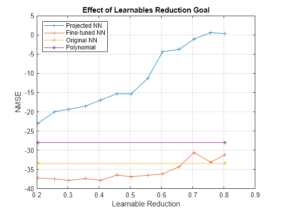
Visualize the effect of the different settings of the learnables reduction goal in a plot. The graphs show that an increase in learnable reduction has a corresponding decrease in the NMSE. A learnable reduction value of around 65% shows a slight decrease in explained variance and a better NMSE than the original neural network.

figure
plot(learnablesReduction,nmseProjectedVec,'+-')
hold on
plot(learnablesReduction,nmseFineTunedVec,'+-')
plot(learnablesReduction([1,end]),nmseOriginal*[1 1],'*-')
plot(learnablesReduction([1,end]),nmseMPDPD*[1 1],'*-')
hold off
grid on
ylabel("NMSE")
legend("Projected NN","Fine-tuned NN","Original NN","Polynomial",Location="northwest")
xlabel("Learnable Reduction")
title("Effect of Learnables Reduction Goal")

Train Final Compressed and Fine-Tuned Network

Compress and fine-tune the DPD neural network for a target compression ratio of 65%.

[netProjected,info] = compressNetworkUsingProjection(netOriginal,npca, ...
  LearnablesReductionGoal=0.65, ...
  VerbosityLevel="off", ...
  LayerNames=["linear1","linear2","linear3"], ...
  UnpackProjectedLayers=true);
info

info = struct with fields:
    LearnablesReduction: 0.6560
      ExplainedVariance: 0.9780
             LayerNames: ["linear1"    "linear2"    "linear3"]

options.MaxEpochs = 150;
options.Verbose = true;
if trainNow
  netFineTunedFinal = trainnet(inputMtxTrain,outputMtxTrain,netProjected,"mse",options);
else
  load savedFineTunedNet30_08Red65.mat netFineTunedFinal
end

Pass the signal through the projected and fine-tuned NN-DPD and calculate the NMSE.

dpdOutNN = predict(netProjected,inputMtxTest);
dpdOutNN = double(complex(dpdOutNN(:,1),dpdOutNN(:,2)));
dpdOutNN = dpdOutNN/scalingFactor;
paOutputNNProjected = pa(dpdOutNN);
nmseProjected = helperNMSE(txWaveTest,paOutputNNProjected);

dpdOutNN = predict(netFineTunedFinal,inputMtxTest);
dpdOutNN = double(complex(dpdOutNN(:,1),dpdOutNN(:,2)));
dpdOutNN = dpdOutNN/scalingFactor;
paOutputNNFineTuned = pa(dpdOutNN);
nmseFineTuned = helperNMSE(txWaveTest,paOutputNNFineTuned);

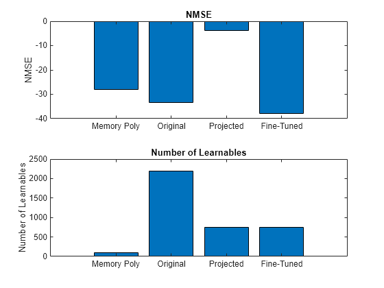
Compare the NMSE and the number of learnables of each network in a bar chart. To calculate the number of learnables of each network, use the numLearnables function, listed in the Number of Learnables Function section of the example. The fine-tuned network performs even better than the original network. The gain in performance might be due to noise generated by unnecessary connections in the network. Removing these connection enables the network to better implement a DPD. Starting with a smaller number of neurons in the original network does not result in a similar performance as the fine-tuned network.

figure
tiledlayout("vertical")
nexttile
bar([nmseMPDPD nmseOriginal nmseProjected nmseFineTuned])
xticklabels(["Memory Poly" "Original" "Projected" "Fine-Tuned"])
title("NMSE")
ylabel("NMSE")
nexttile
bar([memDepth+(memDepth*memDepth*(nonlinearDegree-1)) numLearnables(netOriginal) ...
  numLearnables(netProjected) numLearnables(netProjected)])
xticklabels(["Memory Poly" "Original" "Projected"  "Fine-Tuned"])
ylabel("Number of Learnables")
title("Number of Learnables")

Results and Discussions

Compare the compressed and fine-tuned DPD neural network with the original neural network and the memory polynomial implementation. First, list the estimated number of learnables, number of operations, and parameter memory in MBytes.

metricsOriginal = estimateNetworkMetrics(netOriginal);
summaryMetricsOriginal = metricsOriginal(:,[1 3 4 5])

summaryMetricsOriginal=4×4 table
      LayerName       NumberOfLearnables    NumberOfOperations    ParameterMemory (MB)
    ______________    __________________    __________________    ____________________

    "linear1"                930                   1800                 0.0035477     
    "linear2"                744                   1440                 0.0028381     
    "linear3"                475                    912                  0.001812     
    "linearOutput"            40                     76                0.00015259

metricsFineTuned = estimateNetworkMetrics(netFineTuned);
summaryMetricsFineTuned = metricsFineTuned(:,[1 3 4 5])

summaryMetricsFineTuned=7×4 table
        LayerName         NumberOfLearnables    NumberOfOperations    ParameterMemory (MB)
    __________________    __________________    __________________    ____________________

    "linear1_proj_in"             62                   120                 0.00023651     
    "linear1_proj_out"            90                   120                 0.00034332     
    "linear2_proj_in"             62                   120                 0.00023651     
    "linear2_proj_out"            72                    96                 0.00027466     
    "linear3_proj_in"             50                    96                 0.00019073     
    "linear3_proj_out"            57                    76                 0.00021744     
    "linearOutput"                40                    76                 0.00015259

Calculate the total number of MACs and parameter memory for all three structures.

totalNumMACsFinetuned = sum(metricsFineTuned.NumberOfMACs);
totalNumMACsOriginal = sum(metricsOriginal.NumberOfMACs);
totalMemoryOriginal = sum(metricsOriginal.("ParameterMemory (MB)"))*1e6;
totalMemoryFineTuned = sum(metricsFineTuned.("ParameterMemory (MB)"))*1e6;
totalNumMACsMP = memDepth*(memDepth+(nonlinearDegree-1)*(memDepth-1));
totalMemoryMP = memDepth*(memDepth+(nonlinearDegree-1)*(memDepth-1))*4*2;

Display the results. The original neural network DPD provides about the same NMSE with about 20 times more MACs and 10 times more memory as compared to the memory polynomial DPD. The compressed and fine-tuned network provides more than 8 dB improvement in NMSE with about 1/3rd of the MACs and 1/3 of memory of the original network. When compared to the memory polynomial DPD, the compressed and fine-tuned DPD provides 8 dB improvement in NMSE while increasing the number of MACs by six times and memory by three times, which is better than the results reported in [1].

figure
tiledlayout("vertical")
nexttile
bar([nmseMPDPD nmseOriginal nmseFineTuned])
xticklabels(["Memory Poly" "Original" "Fine-Tuned"])
title("NMSE")
ylabel("NMSE")
nexttile
bar([totalNumMACsMP totalNumMACsOriginal totalNumMACsFinetuned])
xticklabels(["Memory Poly" "Original" "Fine-Tuned"])
ylabel("Number of MACs")
title("Number of MACs")
nexttile
bar([totalMemoryMP totalMemoryOriginal totalMemoryFineTuned])
xticklabels(["Memory Poly" "Original" "Fine Tuned"])
ylabel("Memory")
title("Memory")

Further Exploration

Try a different number of neurons for the original network and then compress and fine-tune it. Also, try different network structures, such as recurrent neural networks.

References

[1] Wu, Yibo, Ulf Gustavsson, Alexandre Graelli Amat, and Henk Wymeersch. “Residual Neural Networks for Digital Predistortion.” In GLOBECOM 2020 - 2020 IEEE Global Communications Conference, 01–06. Taipei, Taiwan: IEEE, 2020. https://doi.org/10.1109/GLOBECOM42002.2020.9322327.

Helper Functions

Number of Learnables

function n = numLearnables(dlnet)
arguments
  dlnet dlnetwork
end
n = sum(cellfun(@numel,dlnet.Learnables.Value));
end

Generate Oversampled OFDM Signals

Generate OFDM-based signals to excite the PA. This example uses a 5G-like OFDM waveform. Set the bandwidth of the signal to 100 MHz. Choosing a larger bandwidth signal causes the PA to introduce more nonlinear distortion and yields greater benefit from the addition of the DPD. Generate six OFDM symbols, where each subcarrier carries a 16-QAM symbol, by using the helperNNDPDGenerateOFDM function. Save the 16-QAM symbols as a reference to calculate the EVM performance. To capture the effects of higher order nonlinearities, the example oversamples the PA input by a factor of 5.

function [txWaveTrain,txWaveVal,txWaveTest,ofdmParams] = generateOversampledOFDMSignals
bw = 100e6;       % Hz
symPerFrame = 6;  % OFDM symbols per frame
M = 16;           % Each OFDM subcarrier contains a 16-QAM symbol
osf = 5;          % oversampling factor for PA input

% OFDM parameters
ofdmParams = helperOFDMParameters(bw,osf);

% OFDM with 16-QAM in data subcarriers
rng(123)
[txWaveTrain] = helperNNDPDGenerateOFDM(ofdmParams,symPerFrame,M);
[txWaveVal] = helperNNDPDGenerateOFDM(ofdmParams,symPerFrame,M);
[txWaveTest] = helperNNDPDGenerateOFDM(ofdmParams,symPerFrame,M);
end