Experiment Manager
Create and run experiments to train and compare deep learning networks
Description
You can use the Experiment Manager app to create deep learning experiments to train networks under different training conditions and compare the results. For example, you can use Experiment Manager to:
Sweep through a range of hyperparameter values, use Bayesian optimization to find optimal training options, or randomly sample hyperparameter values from probability distributions. The Bayesian optimization and random sampling strategies require Statistics and Machine Learning Toolbox™.
Use the built-in function
trainnetor define your own custom training function.Compare the results of using different data sets or test different deep network architectures.
To set up your experiment quickly, you can start with a preconfigured template. The experiment templates support workflows that include image classification and regression, sequence classification, audio classification, signal processing, semantic segmentation, and custom training loops.
The Experiment Browser panel displays the hierarchy of experiments and results in a project. The icon next to the experiment name indicates its type.
 — Built-in training experiment that uses the
trainnettraining function — Custom training experiment that uses a custom
training function
— Custom training experiment that uses a custom
training function — General-purpose experiment that uses a user-authored
experiment function
— General-purpose experiment that uses a user-authored
experiment function
This page contains information about built-in and custom training experiments for Deep Learning Toolbox™. For general information about using the app, see Experiment Manager. For information about using Experiment Manager with the Classification Learner and Regression Learner apps, see Experiment Manager (Statistics and Machine Learning Toolbox).
Required Products
Use Deep Learning Toolbox to run built-in or custom training experiments for deep learning and to view confusion matrices for these experiments.
Use Statistics and Machine Learning Toolbox to run custom training experiments for machine learning and experiments that use Bayesian optimization.
Use Parallel Computing Toolbox™ to run multiple trials at the same time or a single trial on multiple GPUs, on a cluster, or in the cloud. For more information, see Run Experiments in Parallel.
Use MATLAB® Parallel Server™ to offload experiments as batch jobs in a remote cluster. For more information, see Offload Experiments as Batch Jobs to a Cluster.

Open the Experiment Manager App
MATLAB Toolstrip: On the Apps tab, under MATLAB, click the Experiment Manager icon.
MATLAB command prompt: Enter
experimentManager.
For general information about using the app, see Experiment Manager.
Examples
Quickly set up an experiment using a preconfigured experiment template.
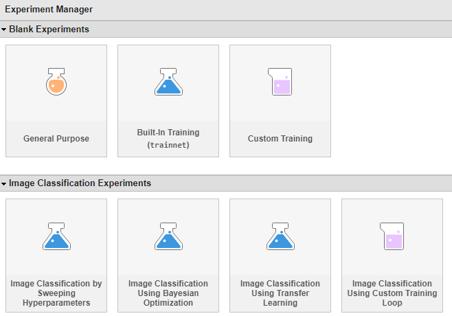
Open the Experiment Manager app. In the dialog box, you can create a new project or open an example from the documentation. Under New, select Blank Project.
In the next dialog box, you can open a blank experiment template or one of the preconfigured experiment templates to support your AI workflow. For example, under Image Classification Experiments, select the preconfigured template Image Classification by Sweeping Hyperparameters.
Specify the name and location for the new project. Experiment Manager opens a new experiment in the project.
The experiment is a built-in training experiment that uses the trainnet
training function, indicated by the ![]() icon.
icon.
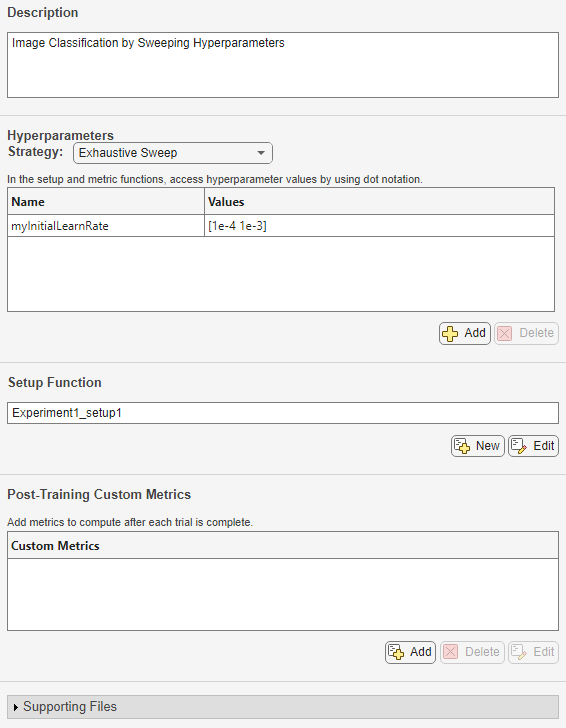
The experiment definition tab displays the description, hyperparameters, setup function, post-training custom metrics, and supporting files that define the experiment. You can modify these parameters to quickly set up your experiment, and then run the experiment.
For information about how to run the experiment and compare results after you configure the experiment parameters, see Experiment Manager.
Set up an experiment that trains using the trainnet
function and exhaustive hyperparameter sweep. Built-in training experiments support
workflows such as image, sequence, time-series, or feature classification and
regression.
Open the Experiment Manager app. In the dialog box, you can create a new project or open an example from the documentation. Under New, select Blank Project.
In the next dialog box, you can open a blank experiment template or one of the
preconfigured experiment templates to support your AI workflow. Under Blank Experiments, select the blank template Built-In Training (trainnet).
The experiment is a built-in training experiment that uses the
trainnet training function, indicated by the ![]() icon.
icon.
The experiment definition tab displays the description, hyperparameters, setup function, post-training custom metrics, and supporting files that define the experiment. When starting with a blank experiment template, you must manually configure these parameters. If you prefer a template with some preconfigured parameters, select one of the preconfigured built-in training templates instead from the Experiment Manager dialog box.

Configure the experiment parameters.
Description — Enter a description of the experiment.
Hyperparameters — Specify the strategy as
Exhaustive Sweepto use every combination of the hyperparameter values. Then, define the hyperparameters to use for your experiment. For more information about choosing and configuring the parameter exploration strategy, see Choose Strategy for Exploring Experiment Parameters.For example, for Evaluate Deep Learning Experiments by Using Metric Functions, the strategy is
Exhaustive Sweepand the hyperparameters areInitialLearnRateandMomentum.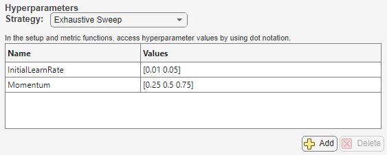
Setup Function — Configure training data, network architecture, loss function, and training options using one of the Setup Function Signatures. The setup function input is a structure with fields from the Hyperparameters table. The output must match the input of the
trainnetfunction.For example, for Evaluate Deep Learning Experiments by Using Metric Functions, the setup function accesses the structure of hyperparameters and returns the inputs to the training function. The setup function is defined in a file named
ClassificationExperiment_setup.mlx.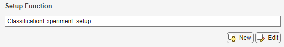
Post-Training Custom Metrics — Compute metrics after each trial to display in the results table. To create the custom metric function, click the Add button in the Post-Training Custom Metrics section. Then, select the metric in the table and click Edit to open and modify the function in the MATLAB Editor. To determine the best combination of hyperparameters for your experiment, inspect the values of these metrics in the results table.
For example, for Evaluate Deep Learning Experiments by Using Metric Functions, the post-training custom metrics are specified by the functions
OnesAsSevensandSevensAsOnes. The functions are defined in files namedOnesAsSevens.mlxandSevensAsOnes.mlx. The results table displays these metrics.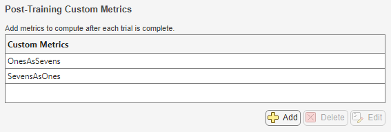
For information about how to run the experiment and compare results after you configure the experiment parameters, see Experiment Manager.
Set up an experiment that trains using the trainnet
function and Bayesian optimization. Built-in training experiments support workflows such
as image, sequence, time-series, or feature classification and regression.
Open the Experiment Manager app. In the dialog box, you can create a new project or open an example from the documentation. Under New, select Blank Project.
In the next dialog box, you can open a blank experiment template or one of the
preconfigured experiment templates to support your AI workflow. Under Blank Experiments, select the blank template Built-In Training (trainnet).
The experiment is a built-in training experiment that uses the
trainnet training function, indicated by the ![]() icon.
icon.
The experiment definition tab displays the description, hyperparameters, setup function, post-training custom metrics, and supporting files that define the experiment. When starting with a blank experiment template, you must manually configure these parameters. If you prefer a template with some preconfigured parameters, select one of the preconfigured built-in training templates instead from the Experiment Manager dialog box.
Configure the experiment parameters.
Description — Enter a description of the experiment.
Hyperparameters — Specify the strategy as
Bayesian
                    Optimization
(Statistics and Machine Learning Toolbox). Specify the hyperparameters as two-element vectors that give the lower bound and upper bound or as an array of strings or a cell array of character vectors that list the possible values of the hyperparameter. The experiment optimizes the specified metric and automatically determines the best combination of hyperparameters for your experiment. Then, specify the maximum time, maximum number of trials, and any advanced options for Bayesian optimization. For more information about choosing and configuring the parameter exploration strategy, see Choose Strategy for Exploring Experiment Parameters.For example, for Tune Experiment Hyperparameters by Using Bayesian Optimization, the strategy is
Bayesian Optimization. The hyperparameter names areSectionDepth,InitialLearnRate,Momentum, andL2Regularization. The maximum number of trials is 30.
Setup Function — Configure training data, network architecture, loss function, and training options using one of the Setup Function Signatures. The setup function input is a structure with fields from the Hyperparameters table. The output must match the input of the
trainnetfunction.For example, for Tune Experiment Hyperparameters by Using Bayesian Optimization, the setup function accesses the structure of hyperparameters and returns the inputs to the training function. The setup function is defined in a file named
BayesOptExperiment_setup.mlx.
Post-Training Custom Metrics — Choose the optimization direction and a standard training or validation metric (such as accuracy, RMSE, or loss) or a custom metric from the table. The output of a metric function must be a numeric, logical, or string scalar.
For example, for Tune Experiment Hyperparameters by Using Bayesian Optimization, the post-training custom metric is specified by a function
ErrorRate. The function is defined in a file namedErrorRate.mlx. The experiment minimizes this metric.
For information about how to run the experiment and compare results after you configure the experiment parameters, see Experiment Manager.
Set up an experiment that trains using a custom training function and creates custom visualizations.
Custom training experiments support workflows that require a training function other
than trainnet. These workflows include:
Training a network that is not defined by a layer graph
Training a network using a custom learning rate schedule
Updating the learnable parameters of a network by using a custom function
Training a generative adversarial network (GAN)
Training a twin neural network
Open the Experiment Manager app. In the dialog box, you can create a new project or open an example from the documentation. Under New, select Blank Project.
In the next dialog box, you can open a blank experiment template or one of the preconfigured experiment templates to support your AI workflow. Under Blank Experiments, select the blank template Custom Training.
The experiment is a custom training experiment that uses a custom training function,
indicated by the ![]() icon.
icon.
The experiment definition tab displays the description, hyperparameters, training function, and supporting files that define the experiment. When starting with a blank experiment template, you must manually configure these parameters. If you prefer a template with some preconfigured parameters, select one of the preconfigured custom training templates instead from the Experiment Manager dialog box.

Configure the experiment parameters.
Description — Enter a description of the experiment.
Hyperparameters — Specify the strategy as
Exhaustive SweeporBayesian Optimization(Statistics and Machine Learning Toolbox), and then define the hyperparameters to use for your experiment. Exhaustive sweep uses every combination of the hyperparameter values, while Bayesian optimization optimizes the specified metric and automatically determines the best combination of hyperparameters for your experiment. For more information about choosing and configuring the parameter exploration strategy, see Choose Strategy for Exploring Experiment Parameters.For example, for Run a Custom Training Experiment for Image Comparison, the strategy is
Exhaustive Sweepand the hyperparameters areWeightsInitializerandBiasInitializer.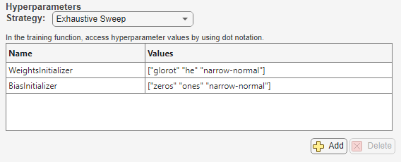
Training Function — Configure training data, network architecture, training procedure, and custom visualizations. Experiment Manager saves the output of this function, so you can export it to the MATLAB workspace when the training is complete. The training function input is a structure with fields from the Hyperparameters table and an
experiments.Monitorobject. Use this object to track the progress of the training, update information fields in the results table, record values of the metrics used by the training, and produce plots.For example, for Run a Custom Training Experiment for Image Comparison, the training function accesses the structure of hyperparameters and returns the a structure that contains the trained network. The training function implements a custom training loop to train a twin neural network, and the function is defined in a file in the project named
ImageComparisonExperiment_training.mlx.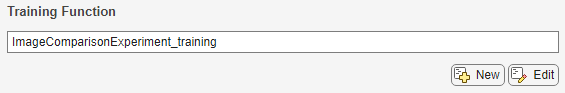
The training function also creates a visualization
Test
                    Images
to display pairs of training images when training is complete.
For information about how to run the experiment and compare results after you configure the experiment parameters, see Experiment Manager.
You can decrease the run time of some experiments if you have Parallel Computing Toolbox or MATLAB Parallel Server.
By default, Experiment Manager runs one trial at a time. If you have Parallel Computing Toolbox, you can run multiple trials at the same time or run a single trial on multiple GPUs, on a cluster, or in the cloud. If you have MATLAB Parallel Server, you can also offload experiments as batch jobs in a remote cluster so that you can continue working or close your MATLAB session while your experiment runs.
In the Experiment Manager toolstrip, in the
Execution section, use the Mode list to
specify an execution mode. If you select the Batch Sequential
or Batch Simultaneous execution mode, use the
Cluster list and Pool Size field in the
toolstrip to specify your cluster and pool size.
For more information, see Run Experiments in Parallel or Offload Experiments as Batch Jobs to a Cluster.
Related Examples
- Compare Classification Network Architectures Using Experiment
- Compare Dropout Probabilities and Filter Configurations for Image Regression Using Experiment
- Evaluate Deep Learning Experiments by Using Metric Functions
- Tune Experiment Hyperparameters by Using Bayesian Optimization
- Use Bayesian Optimization in Custom Training Experiments
- Try Multiple Pretrained Networks for Transfer Learning
- Experiment with Weight Initializers for Transfer Learning
- Audio Transfer Learning Using Experiment Manager
- Choose Training Configurations for LSTM Using Bayesian Optimization
- Run a Custom Training Experiment for Image Comparison
- Use Experiment Manager to Train Generative Adversarial Networks (GANs)
- Custom Training with Multiple GPUs in Experiment Manager
More About
Tips
To visualize and build a network, use the Deep Network Designer app.
To reduce the size of your experiments, discard the results and visualizations of any trial that is no longer relevant. In the Actions column of the results table, click the Discard button
 for the trial.
In your setup function, access the hyperparameter values using dot notation. For more information, see Structure Arrays.
For networks containing batch normalization layers, if the
BatchNormalizationStatisticstraining option ispopulation, Experiment Manager displays final validation metric values that are often different from the validation metrics evaluated during training. The difference in values is the result of additional operations performed after the network finishes training. For more information, see Batch Normalization Layer.
Version History
Introduced in R2020aIn the Experiment Manager toolstrip, the Restart list replaces the Restart All Canceled button. To restart multiple trials of your experiment, open the Restart list, select one or more restarting criteria, and click Restart
 . The restarting criteria include
 All Canceled,All Stopped,All Error, andAll Discarded.During training, the results table displays the intermediate values for standard training and validation metrics for built-in training experiments. These metrics include loss, accuracy (for classification experiments), and root mean squared error (for regression experiments).
In built-in training experiments, the Execution Environment column of the results table displays whether each trial of a built-in training experiment runs on a single CPU, a single GPU, multiple CPUs, or multiple GPUs.
To discard the training plot, confusion matrix, and training results for trials that are no longer relevant, in the Actions column of the results table, click the Discard button
.
In the Experiment Manager toolstrip, the Mode list replaces the Use Parallel button.
To run one trial of the experiment at a time, select
Sequentialand click Run.To run multiple trials at the same time, select
Simultaneousand click Run.To offload the experiment as a batch job, select
Batch SequentialorBatch Simultaneous, specify your cluster and pool size, and click Run.
Manage experiments using new Experiment Browser context menu options:
To add a new experiment to a project, right-click the name of the project and select New Experiment.
To create a copy of an experiment, right-click the name of the experiment and select Duplicate.
Specify hyperparameter values as cell arrays of character vectors. In previous releases, Experiment Manager supported only hyperparameter specifications using scalars and vectors with numeric, logical, or string values.
To stop, cancel, or restart a trial, in the Action column of the results table, click the Stop
 , Cancel
  , or Restart
  buttons. In previous releases, these buttons were
located in the Progress column. Alternatively, you can right-click
the row for the trial and, in the context menu, select Stop, Cancel, or Restart.
buttons. In previous releases, these buttons were
located in the Progress column. Alternatively, you can right-click
the row for the trial and, in the context menu, select Stop, Cancel, or Restart.When an experiment trial ends, the Status column of the results table displays one of these reasons for stopping:
Max epochs completedMet validation criterionStopped by OutputFcnTraining loss is NaN
To sort annotations by creation time or trial number, in the Annotations panel, use the Sort By list.
After training completes, save the contents of the results table as a
tablearray in the MATLAB workspace by selecting Export > Results Table.To export the training information or trained network for a stopped or completed trial, right-click the row for the trial and, in the context menu, select Export Training Information or Export Trained Network.
See Also
Apps
- Experiment Manager | Experiment Manager (Statistics and Machine Learning Toolbox) | Deep Network Designer