initial
System response to initial states of state-space model
Syntax
Description
For state-space and sparse state-space models, initial
computes the unforced system response y to initial states
xinit.
Continuous time:
Discrete time:
This is the system response when u(t) is maintained at the offset value u0.
For linear time-varying or linear parameter-varying state-space models,
initial computes the response with initial state
xinit, initial parameters
pinit (LPV models), and input held to the offset
value (u(t) =
u0(t) or u(t) =
u0(t,p), which corresponds to the initial condition response of the local linear
dynamics.
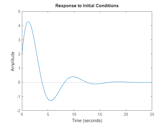
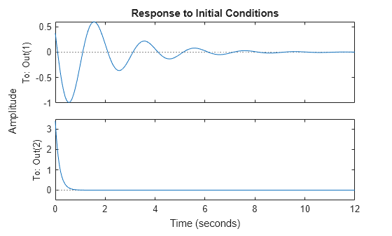
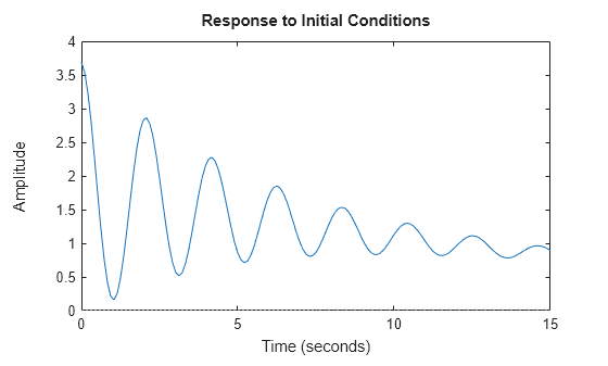
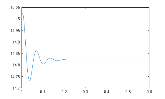
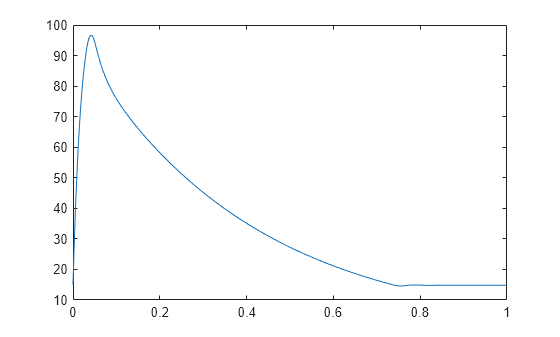
initial(___) plots the initial condition response of
sys with default plotting options for all of the previous input
argument combinations. For more plot customization options, use initialplot.
To plot responses for multiple dynamic systems on the same plot, you can specify
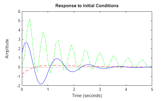
sysas a comma-separated list of models. For example,initial(sys1,sys2,sys3)plots the responses for three models on the same plot.To specify a color, line style, and marker for each system in the plot, specify a
LineSpecvalue for each system. For example,initial(sys1,LineSpec1,sys2,LineSpec2)plots two models and specifies their plot style. For more information on specifying aLineSpecvalue, seeinitialplot.
Examples
Input Arguments
Output Arguments
Tips
When you need additional plot customization options, use
initialplotinstead.Plots created using
initialdo not support multiline titles or labels specified as string arrays or cell arrays of character vectors. To specify multiline titles and labels, use a single string with anewlinecharacter.initial(sys) title("first line" + newline + "second line");
Version History
Introduced before R2006aSee Also
initialplot | impulse | lsim | Linear System Analyzer | step

