sminreal
R2026bEliminates structurally disconnected states, delays, and blocks
Syntax
Description
Use sminreal to eliminate the states of a state-space model
that do not affect the input-output response of the model.
In state-space models, sminreal eliminates all states and internal
delay signals that are structurally disconnected from the inputs and outputs. The simplified
model is structurally minimal, that is, generically minimal when randomizing the nonzero
entries of state matrices.
In generalized models, sminreal further eliminates all tunable or
uncertain blocks that are structurally disconnected from the inputs and outputs.
In gridded LTV and LPV models, sminreal eliminates states and
internal delays that are structurally disconnected for all models in the
grid. The remaining states and internal delay signals are the same for all models across the
grid.
msys = sminreal(sys)sys that do not affect
the input-output response and returns the simplified model msys. All of
the states of the resulting state-space model msys are also states of
sys and the input/output response of msys is
equivalent to that of sys.
msys = sminreal(sys,info)info
must be preserved. Here, info is typically a matrix containing initial
conditions. Note that the presence of offsets and initial conditions influences the
input-to-state map and therefore affects which states can be safely removed.
[
also returns the updated msys,xkeep,info] = sminreal(___)info structure, containing updated projection
and initial condition information to reflect the transformation performed by
sminreal, as last output. Here, the info input
argument is typically a structure containing both initial condition and projection matrices
to propagate through the transformation. For more information on projector matrices, see
Spectral Projector Matrices.
When you use "consistent", xkeep is always a
vector, and the info output argument is always a single
structure.
Examples
This example shows how to use sminreal to perform a state-consistent state elimination in a state-space array.
Load the model.
load ssarray.mat
size(asys)
6x1 array of state-space models. Each model has 1 outputs, 1 inputs, and 3 states.
Perform the state-elimination. With "consistent" option, the function removes only those states and delays that do not contribute to the I/O map for all models.
[rsys,xkeep] = sminreal(asys,"consistent");
size(rsys)
6x1 array of state-space models. Each model has 1 outputs, 1 inputs, and 1 states.
xkeep
xkeep = 3×1 logical array

    0
    1
    0
sminreal eliminates first and third states from all models in the array. For state-space arrays with uniform state dimension, sminreal eliminates states and delays that are structurally nonminimal for all models in the array, taking offsets into account.
step(asys,rsys,'r--')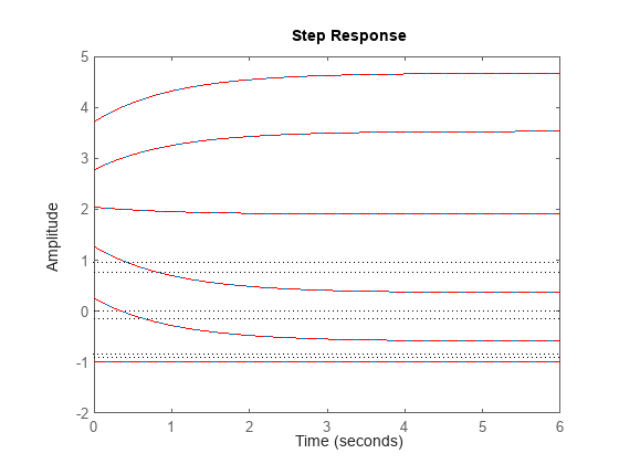
As you can see, the responses are identical.
In this example, you simplify two state-space models with initial conditions. The first model has unobservable states, while the second model has uncontrollable states.
Unobservable states and delays can always be removed. On the other hand, uncontrollable states can be removed only when their initial value matches the state offset. As a result, the output trajectories of the original and simplified models match for all initial states in the subspace spanned by the initial condition.
Simplify model with unobservable states
Create two random state space subsystems.
h1 = rss(3);
h2 = rss(2);
Assemble the subsystems in parallel.
sys = [h1; h2];
Create an initial condition vector.
x0 = randn(5,1);
Create a copy of sys in which the second output is discarded.
sys11 = sys(1,1);
In sys11, the states from h2 are unobservable:
rank(obsv(sys11))
ans =
3
Obtain the reduced system rsys by simplifying sys11.
[rsys,xkeep,info] = sminreal(sys11,x0);
rsys matches h1:
isequal(rsys,h1)
ans = logical
   1
Display the initial condition.
info.InitialCondition
ans = 3×1

    0.3714
   -0.2256
    1.1174
You can also obtain it as:
info.PX'*x0
ans = 3×1

    0.3714
   -0.2256
    1.1174
As expected it matches the initial conditions in the observable space:
x0(1:3)
ans = 3×1

    0.3714
   -0.2256
    1.1174
Simplify model with uncontrollable states
Assemble the subsystems in series.
sys = [h1 h2];
Create a copy of sys in which the second input is discarded.
sys11 = sys(1,1);
In sys11, the states from h2 are uncontrollable:
rank(ctrb(sys11))
ans =
3
Try to reduce the system.
[rsys,xkeep,info] = sminreal(sys11,x0);
rsys matches the original system sys11:
isequal(rsys,sys11)
ans = logical
   1
The uncontrollable states were not removed because they have a non-zero initial condition.
Now zero out the initial conditions in the uncontrollable dimensions.
x0(4:5) = [0 0]';
Obtain the reduced system rsys by simplifying sys11.
[rsys,xkeep,info] = sminreal(sys11,x0);
Now rsys matches h1:
isequal(rsys,h1)
ans = logical
   1
Display the initial condition.
info.InitialCondition
ans = 3×1

    0.3714
   -0.2256
    1.1174
Input Arguments
Output Arguments
Tips
The model resulting from sminreal(sys) is not necessarily minimal, and may
have a higher order than one resulting from minreal(sys). However,
sminreal(sys) retains a subset of the original states of
sys, while, in general, minreal(sys) does
not.
References
[1] Heinkenschloss, M., T. Reis, and A. C. Antoulas. “Balanced Truncation Model Reduction for Systems with Inhomogeneous Initial Conditions.” Automatica 47, no. 3 (2011): 559–64. https://doi.org/10.1016/j.automatica.2010.12.002.

