MIMO Control System with Fixed and Tunable Components
This example shows how to build a MIMO control system using connect to build a dynamic system model representing a block diagram with both fixed components (Numeric Linear Time Invariant (LTI) Models) and tunable components (Control Design Blocks). You can use the techniques of this example to construct a model from any type of dynamic system models or elements.
Consider the two-input, two-output control system of the following illustration.
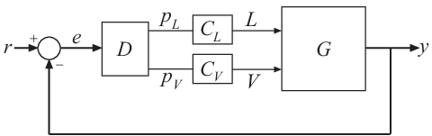
The plant G is a distillation column with two inputs and two outputs. The plant inputs are the reflux L and boilup V. The two outputs are the concentrations of two chemicals, represented by the vector signal y = [y(1),y(2)]. For this example, suppose that the plant model is as follows.
The vector setpoint signal r = [r(1),r(2)] specifies the desired concentrations of the two chemicals. The vector error signal e represents the input to D, a static 2-by-2 decoupling matrix. CL and CV represent independent PI controllers that control the two inputs of G.
Build the Block Diagram
To create a two-input, two-output dynamic system model representing this block diagram, first create LTI models representing each component. For this example, use a state-space model for the plant. Set the InputName and OutputName properties of the plant model using the signal names from the diagram.
s = tf('s');
G = [87.8 -86.4 ; 108.2 -109.6]/(75*s+1);
G.InputName = {'L','V'};
G.OutputName = 'y';
In this example, the two inputs are individually named. You can also assign a single name to a multi-channel input or output and allow the software to expand the name. For instance, examine the plant output names.
G.OutputName
ans = 2×1 cell
    {'y(1)'}
    {'y(2)'}
For this example, represent the PI controllers and the decoupling matrix with tunable control design blocks.
D = tunableGain('Decoupler',eye(2));
D.InputName = 'e';
D.OutputName = {'pL','pV'};

C_L = tunablePID('C_L','pi');
C_L.InputName = 'pL';
C_L.OutputName = 'L';

C_V = tunablePID('C_V','pi');
C_V.InputName = 'pV';
C_V.OutputName = 'V';
When you are assigning input and output names to a model, you can use the shortcuts u and y to set the InputName and OutputName properties, respectively. For example, the following is an alternative way to specify the input and output names of the controller C_V.
C_V.u = 'pV';
C_V.y = 'V';
Create an element to represent the summing junction using the sumblk command. The summing junction in this diagram takes the difference between the vector signals r and y and produces the output e. Thus, the summing junction has the formula e = r – y.
Sum = sumblk('e = r - y',2);The input argument 2 tells sumblk that the inputs and outputs of Sum are each vector signals of length 2. The software therefore automatically expands the signal names. For instance, examine the input names.
Sum.InputName
ans = 4×1 cell
    {'r(1)'}
    {'r(2)'}
    {'y(1)'}
    {'y(2)'}
Next, use connect to join all the components to build the closed-loop system from r to y.
CL = connect(G,D,C_L,C_V,Sum,'r','y');
The arguments to the connect function include all the components of the closed-loop system, in any order. connect automatically combines the components using the input and output names to join signals. The last two arguments to connect specify the output and input signals of the closed-loop model, respectively. The resulting genss model CL has two inputs and two outputs, because both r and y are vector signals.
CL
Generalized continuous-time state-space model with 2 outputs, 2 inputs, 4 states, and the following blocks:
  C_L: Tunable PID controller, 1 occurrences.
  C_V: Tunable PID controller, 1 occurrences.
  Decoupler: Tunable 2x2 gain, 1 occurrences.
Model Properties

Type "ss(CL)" to see the current value and "CL.Blocks" to interact with the blocks.
Other System Responses
Suppose that you want to know the response of this system to disturbances at the plant inputs. You can obtain that by building analysis points into the block diagram at the plant inputs. Analysis points are locations in the model where you can inject disturbances or extract responses. With connect, you can directly specify signal locations at which you want to introduce analysis points. To study the system response to disturbance at the plant inputs, insert analysis points at the signal locations L and V.
APs = {'L','V'};
CL_APs = connect(G,D,C_L,C_V,Sum,'r','y',APs);
CL_APs
Generalized continuous-time state-space model with 2 outputs, 2 inputs, 4 states, and the following blocks: CONNECT_AP1: Analysis point, 2 channels, 1 occurrences. C_L: Tunable PID controller, 1 occurrences. C_V: Tunable PID controller, 1 occurrences. Decoupler: Tunable 2x2 gain, 1 occurrences. Model Properties Type "ss(CL_APs)" to see the current value and "CL_APs.Blocks" to interact with the blocks.
You can now use commands like getIOTransfer to extract desired system responses, including those with inputs or outputs at the analysis points. Extract the system response to disturbances injected at the plant inputs.
Td = getIOTransfer(CL_APs,APs,'y');
Td.InputName
ans = 2×1 cell
{'L'}
{'V'}
Td.OutputName
ans = 2×1 cell
    {'y(1)'}
    {'y(2)'}
See Also
connect | sumblk | getIOTransfer