Generate Data and Segment Signals for Transmission System Fault Detection

R2026b

Since R2026b

This example uses:

This example shows how to generate data and segment signals for various fault and failure scenarios in an automotive transmission system. Ensure the simulated data set meets the requirements described in Signal Data Requirements.

Note: This example requires Predictive Maintenance Toolbox™.

Open Transmission System Model

Open the Simulink® model transmissionSystemDataGenerator. This model simulates the transmission system of an automobile under the various fault and failure conditions outlined in Fault and Failure Scenarios. The model is a modification of the Simulink model used in the Using Simulink to Generate Fault Data (Predictive Maintenance Toolbox) example. The model logs vibration and tacho signals using sensors in the Simulink system that can be used to detect faults in an automobile system. Assume that the noise signal added to the vibration signal is a Gaussian signal, where the signal to noise ratio is roughly 26 dB.

mdl = "transmissionSystemDataGenerator";
open_system(mdl);

The transmission casing model uses Simscape™ Driveline™ blocks to model a simple transmission system. The transmission system consists of a torque drive, drive shaft, clutch, and high and low gears connected to an output shaft.

subSystem = "transmissionSystemDataGenerator/Vehicle Transmission System";
open_system(subSystem);

Model Fault Scenarios

In this example, the transmission system has two possible target faults: sensor drift and shaft wear. For each type of fault, compare healthy conditions to conditions where the fault is present.

Sensor Drift Fault

Simulate a sensor drift fault by adding drift to the vibration signal, and observe how the vibration signal changes.

open_system(subSystem + "/Vibration sensor with drift");

First, simulate healthy conditions. Fix a random seed generator, and set a simulation time of 40 seconds.

Seed = 1;
Tstop = 40;
SensorDriftHealthyOutput = sim(mdl,StopTime = num2str(Tstop));

Then, simulate a signal in the presence of sensor drift by setting SDProfile to 1.

SDProfile = 1;
SensorDriftFaultyOutput = sim(mdl,StopTime = num2str(Tstop));

Visualize the vibration signal under healthy and sensor drift conditions.

vSensorDriftHealthy = SensorDriftHealthyOutput.logsout{3}.Values;
vSensorDriftFaulty = SensorDriftFaultyOutput.logsout{3}.Values;
figure
plot(vSensorDriftHealthy.Time,vSensorDriftHealthy.Data)
hold on
plot(vSensorDriftFaulty.Time,vSensorDriftFaulty.Data,Color=[0.8660,0.3290,0])
hold off
title("Vibration")
ylabel("Acceleration")
legend("Healthy","Sensor drift")

Figure contains an axes object. The axes object with title Vibration, ylabel Acceleration contains 2 objects of type line. These objects represent Healthy, Sensor drift.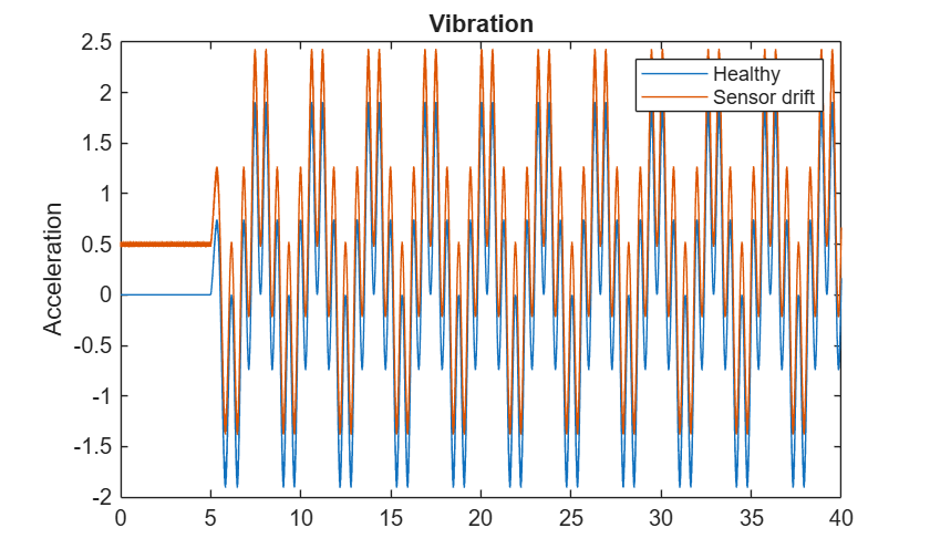

The offset introduced in the vibration signal is constant. In practice, a minor offset might be acceptable, but a larger offset indicates a system fault that needs to be detected.

Visualize the tacho pulses under healthy and sensor drift conditions.

tSensorDriftHealthy = SensorDriftHealthyOutput.logsout{2}.Values;
tSensorDriftFaulty = SensorDriftFaultyOutput.logsout{2}.Values;
figure
tiledlayout(2,1)
nexttile
plot(tSensorDriftHealthy.Time,tSensorDriftHealthy.Data)
title("Tacho Pulses of Healthy Signals")
legend("Drive shaft","Load shaft")
nexttile
plot(tSensorDriftFaulty.Time,tSensorDriftFaulty.Data)
title("Tacho Pulses of Signals with Sensor Drift")
legend("Drive shaft","Load shaft")

Figure contains 2 axes objects. Axes object 1 with title Tacho Pulses of Healthy Signals contains 2 objects of type line. These objects represent Drive shaft, Load shaft. Axes object 2 with title Tacho Pulses of Signals with Sensor Drift contains 2 objects of type line. These objects represent Drive shaft, Load shaft.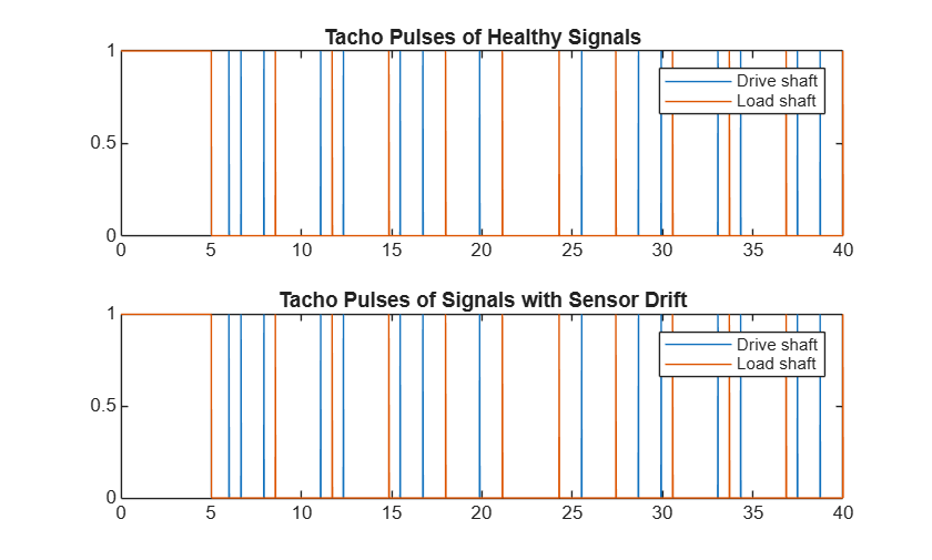

The tacho pulses are identical, indicating that the sensor drift does not affect the times of the shaft rotations.

Shaft Wear Fault

Simulate a shaft wear fault using a variant subsystem that can switch between a healthy output shaft and a worn output shaft. Both systems use Simscape™ elements like Clutch Brake, Damper Axle, and so on. The system simulates a worn output shaft by increasing the damping coefficient in the Damper Axle and the static friction coefficient in the Clutch Brake.

open_system(subSystem + "/Shaft");
open_system(subSystem + "/Shaft/Healthy Output Shaft");
open_system(subSystem + "/Shaft/Worn Output Shaft");

Run a simulation under shaft wear conditions (by setting SWProfile to 1) and under healthy conditions (by setting SWProfile to 0). Because shaft wear is slow to occur, set a simulation time of 120 seconds.

SWProfile = 1;
SDProfile = 0;
Tstop = 120;
ShaftWearFaultyOutput = sim(mdl,StopTime = num2str(Tstop));
SWProfile = 0;
ShaftWearHealthyOutput = sim(mdl,StopTime = num2str(Tstop));

Visualize the vibration signal under healthy and shaft wear conditions.

vShaftWearHealthy = ShaftWearHealthyOutput.logsout{3}.Values;
vShaftWearFaulty = ShaftWearFaultyOutput.logsout{3}.Values;
figure
plot(vShaftWearHealthy.Time,vShaftWearHealthy.Data)
hold on
plot(vShaftWearFaulty.Time,vShaftWearFaulty.Data,Color=[0.8660,0.3290,0])
hold off
title("Vibration")
ylabel("Acceleration")
legend("Healthy","Shaft wear")

Figure contains an axes object. The axes object with title Vibration, ylabel Acceleration contains 2 objects of type line. These objects represent Healthy, Shaft wear.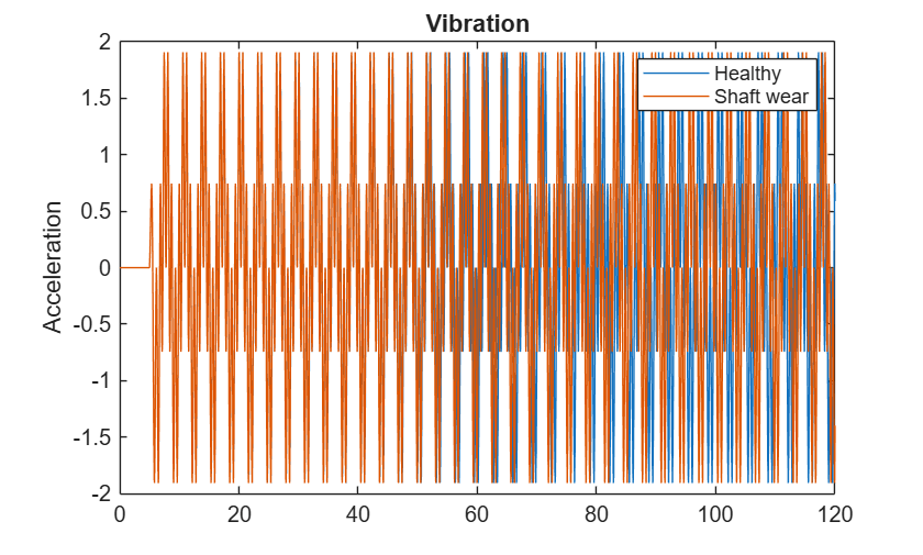

You can see the slow effect of the shaft wear over time.

Visualize the tacho pulses under healthy and shaft wear conditions.

tShaftWearHealthy = ShaftWearHealthyOutput.logsout{2}.Values;
tShaftWearFaulty = ShaftWearFaultyOutput.logsout{2}.Values;
figure
tiledlayout(2,1)
nexttile
plot(tShaftWearHealthy.Time,tShaftWearHealthy.Data)
title("Tacho Pulses of Healthy Signals")
legend("Drive shaft","Load shaft")
nexttile
plot(tShaftWearFaulty.Time,tShaftWearFaulty.Data)
title("Tacho Pulses of Signals with Shaft Wear")
legend("Drive shaft","Load shaft")

Figure contains 2 axes objects. Axes object 1 with title Tacho Pulses of Healthy Signals contains 2 objects of type line. These objects represent Drive shaft, Load shaft. Axes object 2 with title Tacho Pulses of Signals with Shaft Wear contains 2 objects of type line. These objects represent Drive shaft, Load shaft.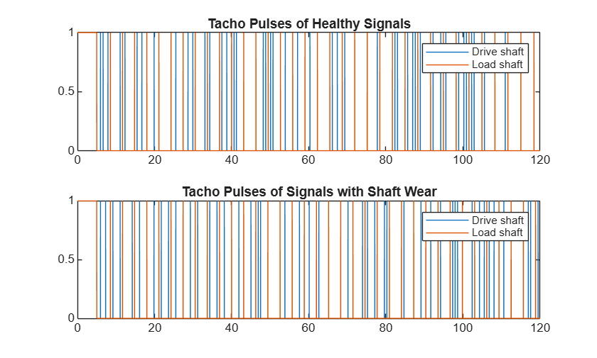

The shaft wear affects the pulse timings of the shaft rotations, although the effect is difficult to detect visually.

Create Signal Windows

Each simulation produces continuous signals spanning the full simulation duration (for example, 310 seconds in production mode). In order to train fault detection models on simulation data, you must first reformat the simulation data. In particular, segment the long signals into non-overlapping 30-second windows. Discard the first 10 seconds of each simulation (transient startup), and split the remaining signal into fixed-length windows. Each window becomes one observation (row) in the data set.

Visualize the division of a sample vibration signal into 30-second windows.

windowLength = 30;
startupDiscard = 10;
% Use the healthy 120s simulation from earlier
signalData = ShaftWearHealthyOutput.logsout{3}.Values;
vSignal = signalData.Data;
tSignal = signalData.Time;
% Discard first 10 seconds
idx = tSignal > startupDiscard;
vSignal = vSignal(idx,:);
tSignal = tSignal(idx,:);
tSignal = tSignal - tSignal(1);
figure
plot(tSignal,vSignal,Color=[0.5 0.5 0.5])
hold on
totalDuration = tSignal(end);
nWindows = floor(totalDuration / windowLength);
colors = lines(nWindows);
for w = 1:nWindows
    tStart = (w-1) * windowLength;
    tEnd = w * windowLength;
    winIdx = tSignal >= tStart & tSignal < tEnd;
    plot(tSignal(winIdx),vSignal(winIdx),Color=colors(w,:))
    xline(tStart,"--k",sprintf("W%d",w),LabelVerticalAlignment="top")
end
hold off
title("Signal Windowing: 30-Second Non-Overlapping Windows")
xlabel("Time (s)")
ylabel("Vibration Acceleration")
subtitle(sprintf("First %ds discarded | %d windows of %ds each", ...
    startupDiscard,nWindows,windowLength))

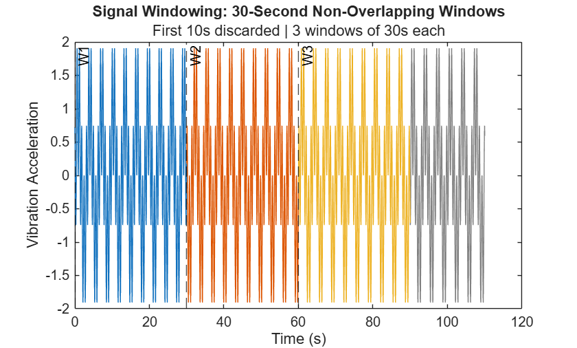
Figure contains an axes object. The axes object with title Signal Windowing: 30-Second Non-Overlapping Windows, xlabel Time (s), ylabel Vibration Acceleration contains 7 objects of type line, constantline.

Each colored segment represents one 30-second window that becomes a single observation in the data set. The attached prepareSignals.m function file allows you to split signals into 30-second windows. During feature extraction, you can compute features (such as mean, root mean square, kurtosis, and so on) independently on each window. For more information, see Extract Features and Partition Data for Transmission System Fault Detection.

To train fault detection models on the data, the split signals must be labeled with the correct fault scenario. Use the following heuristic to determine the presence a sensor drift fault, shaft wear fault, or gear tooth failure:

If $| S D r i f t | > 0.01$ , then a sensor drift fault exists.
If $S h a f t W e a r < 0$ , then a shaft wear fault exists.
If $| T o o t h F a u l t G a i n | > 0.1$ , then a gear tooth failure exists.

Generate Data Using Simulink Model

You can run the attached generateAllScenarioData.m function file to generate data for various fault and failure conditions using the transmissionSystemDataGenerator model. In the code below, set generateData to true. The data generation process can take a long time to run.

When generateData is set to false, the example uses previously saved data instead.

generateData = false;

if generateData
    generateAllScenarioData;
end

Verify Signal Data Requirements

Verify that the generated data satisfies the signal data requirements described in Signal Data Requirements. In particular, sufficient observations must exist for each simulation scenario (at least 200), and all vibration signals must be in the range [-3,3]. Use the helper function helperVerifyRequirements to summarize the results in a table.

verificationTable = helperVerifyRequirements

verificationTable = 9×4 table
          RequirementID                                         Description                                    NumSamples     Result 
    _________________________    __________________________________________________________________________    __________    ________

    "COMPLETENESS_SCENARIO_1"    "Scenario 1: Healthy (no faults, no failure)"                                     400       "PASSED"
    "COMPLETENESS_SCENARIO_2"    "Scenario 2: Sensor drift fault"                                                  200       "PASSED"
    "COMPLETENESS_SCENARIO_3"    "Scenario 3: Shaft wear fault"                                                    200       "PASSED"
    "COMPLETENESS_SCENARIO_4"    "Scenario 4: Sensor drift and shaft wear faults"                                  200       "PASSED"
    "COMPLETENESS_SCENARIO_5"    "Scenario 5: Gear tooth failure"                                                  210       "PASSED"
    "COMPLETENESS_SCENARIO_6"    "Scenario 6: Sensor drift fault and gear tooth failure"                           210       "PASSED"
    "COMPLETENESS_SCENARIO_7"    "Scenario 7: Shaft wear fault and gear tooth failure"                             210       "PASSED"
    "COMPLETENESS_SCENARIO_8"    "Scenario 8: Sensor drift fault, shaft wear fault, and gear tooth failure"        210       "PASSED"
    "VALIDITY"                   "Vibration signals within [-3, 3]"                                               1840       "PASSED"

	Get insights using Copilot

The verification table shows that the generated data set passes all the completeness and validity requirements. You can now extract features from the generated data to train fault detection models.

Helper Function

The helperVerifyRequirements function determines whether the requirements described in Signal Data Requirements are met. The function returns a table (verificationTable) with the results.

function verificationTable = helperVerifyRequirements

minSamplesRequired = 200;
validRange = [-3 3];

supportFileNames = ["faultScenario1","faultScenario2","faultScenario3","faultScenario4", ...
    "faultScenario5","faultScenario6","faultScenario7","faultScenario8"];
scenarioVarNames = ["dataTable_s1","dataTable_s2","dataTable_s3","dataTable_s4", ...
    "dataTable_s5","dataTable_s6","dataTable_s7","dataTable_s8"];

RequirementID = strings(9,1);
Description = strings(9,1);
NumSamples = zeros(9,1);
Result = strings(9,1);

scenarioDescriptions = [
    "Healthy (no faults, no failure)"
    "Sensor drift fault"
    "Shaft wear fault"
    "Sensor drift and shaft wear faults"
    "Gear tooth failure"
    "Sensor drift fault and gear tooth failure"
    "Shaft wear fault and gear tooth failure"
    "Sensor drift fault, shaft wear fault, and gear tooth failure"];

allValid = true;
for k = 1:8
    d = load(matlab.internal.examples.downloadSupportFile("nnet", ...
        "data/transmissionfaults/" + supportFileNames(k) + ".mat"));
    tbl = d.(scenarioVarNames(k));
    nRows = height(tbl);

    RequirementID(k) = sprintf("COMPLETENESS_SCENARIO_%d",k);
    Description(k) = sprintf("Scenario %d: %s",k,scenarioDescriptions(k));
    NumSamples(k) = nRows;

    if nRows >= minSamplesRequired
        Result(k) = "PASSED";
    else
        Result(k) = "FAILED";
    end

    for row = 1:nRows
        vibData = tbl.Vibration{row}.Variables;
        if any(vibData < validRange(1)) || any(vibData > validRange(2))
            allValid = false;
            break;
        end
    end
end

RequirementID(9) = "VALIDITY";
Description(9) = "Vibration signals within [-3, 3]";
NumSamples(9) = sum(NumSamples(1:8));
if allValid
    Result(9) = "PASSED";
else
    Result(9) = "FAILED";
end

verificationTable = table(RequirementID,Description,NumSamples,Result);
end