Physical System Modeling Using LSTM Network in Simulink

This example uses:

This example shows how to create a reduced order model (ROM) that acts as a virtual sensor in a Simulink® model using a long short-term memory (LSTM) neural network.

A ROM is a surrogate for a physical model that allows you to reduce the computation required with an acceptable compromise of the accuracy of the original physical model. For virtual sensor applications, where the model needs to run at high sampling rates in an embedded system, ROMs provide suitable approximations of the original physical system. While there is a variety of techniques for building a ROM, this example builds an LSTM-ROM (a type of ROM that leverages an LSTM network) and uses it in a Simulink model as a set of layer blocks.

To train the LSTM network, the example uses the original model to generate the training data. The trained LSTM in the ROM takes the B and F signals of the load shaft and the control pressure as input and predicts the next value of the B and F signals of the load shaft. After the model is trained, the example creates an LSTM-ROM component and replaces the physical component in the Simulink model with it.

This diagram shows the physical component to replace in the Simulink model.

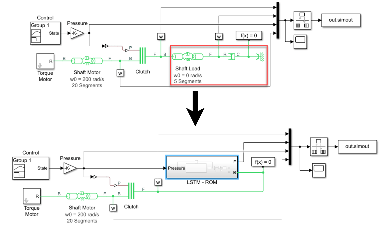
This diagram shows the Simulink model with the physical component replaced by an LSTM-ROM subcomponent.

Training the LSTM network for an LSTM-ROM is a computationally intensive task and can take a long time to run. To speed up the example, the example skips training and loads a pretrained version of the network. To instead train the network, set the doTraining variable to true.

doTraining = false;

Generate Training Data

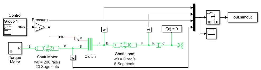
Generate the training data using the Simulink model ex_sdl_flexible_shaft, attached to this example as a supporting file. To access this model, open this example as a live script. This Simulink model simulates a flexible shaft. It has two flexible aluminum shafts modeled using a lumped parameter approach: the motor shaft, consisting of 20 segments, and the load shaft, consisting of 5 segments. Both shafts contain inertias, damping, and stiff torsional springs. At the start of the simulation, the clutch is unlocked and the driven shaft is free. The initial velocity of the motor shaft is set to 200 rad/s and the system starts at steady state. The model uses the pressure applied on the clutch as a control parameter to determine the dynamics of the model.

The Simulink model outputs four values:

Base (B) signal of the load shaft
Follower (F) signal of the load shaft
Control pressure
F signal of the motor shaft

The first three states are used to train the LSTM-ROM. The fourth state is used for evaluating the accuracy of the trained model.

This diagram shows the structure of the model.

The Simulink model depends on the workspace variables stopTime and timeInterval, which specify the final time step and the interval between output time steps of the simulation, respectively. The initial time step of the simulation is 0.

Specify a stop time of 0.2 and a time interval of $5 \times 1 0^{- 5}$ .

stopTime = 0.2;
timeInterval = 5e-5;

The Pressure block of the model depends on the workspace variable maxPressure, which defines the value of the maximum pressure applied on the clutch. Run the model for 20 different equally spaced values of maxPressure between $1 0^{5}$ and $1 0^{6}$ . Collect the output data in the cell array data, where each element corresponds to a time series observation computed with the specified pressure profile.

numObservations = 20;
maxPressures = linspace(1e5,1e6,numObservations);

data = cell(numObservations,1);

for i = 1:numObservations
    maxPressure = maxPressures(i);
    simout = sim("ex_sdl_flexible_shaft");
    data{i} = simout.simout.Data;
end

Extract the time steps of the simulations.

times = simout.simout.Time;
numTimeSteps = length(times);

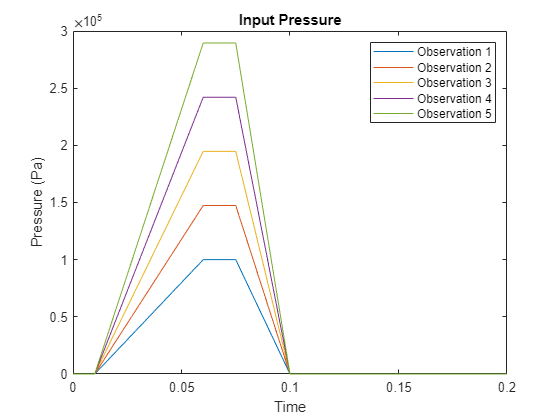
Plot the control pressures of the first five simulations.

figure
for i = 1:5
    pressure = data{i}(:,3);
    plot(times,pressure);
    hold on
end

title("Input Pressure")
legend("Observation " + (1:5))
xlabel("Time")
ylabel("Pressure (Pa)")
hold off

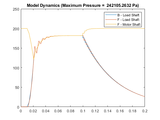
Plot the B and F signals of the load shaft and the F signal of the motor shaft of one of the simulations.

idx = 4;
BLoadShaft = data{idx}(:,1);
FLoadShaft = data{idx}(:,2);
FMotorShaft = data{idx}(:,4);

figure
plot(times,BLoadShaft, ...
    times,FLoadShaft, ...
    times,FMotorShaft)

legend("B - Load Shaft", "F - Load Shaft", "F - Motor Shaft")
title("Model Dynamics (Maximum Pressure =  " + maxPressures(idx) + " Pa)")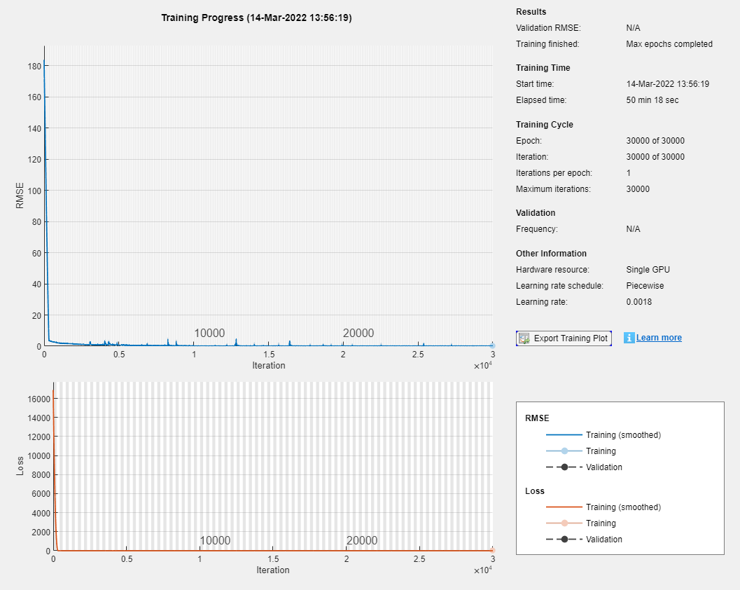

Prepare Data for Training

When you train an LSTM with very long sequences, the accumulation of the gradients computed for each time step can lead to vanishing gradients and cause the training process to converge to a suboptimal result. To prevent the gradients from vanishing, downsample the training data so that the sequences are much shorter without losing too much of the information.

To downsample the data, specify a sample time that is larger than the sample time of the training data. When you export the LSTM network to Simulink as layer blocks, you must specify the same value in the SampleTime name-value argument of exportNetworkToSimulink.

Specify a sample time of $1 0^{- 3}$ .

sampleTime = 1e-3;

Downsample the training data by extracting time steps with a fixed interval given by the sample time divided by the time interval of the simulation.

intervalDownsampled = sampleTime / timeInterval;
timeStepsDownsampled = 1:intervalDownsampled:numTimeSteps;

for i = 1:numObservations
    dataDownsampled{i} = data{i}(timeStepsDownsampled,:);
end

Partition the training data evenly into training and test partitions using the trainingPartitions function, attached to this example as a supporting file. To access this file, open the example as a live script.

[idxTrain,idxTest] = trainingPartitions(numObservations,[0.5 0.5]);

maxPressuresTrain = maxPressures(idxTrain);
maxPressuresTest = maxPressures(idxTest);
dataTrain = dataDownsampled(idxTrain);
dataTest = dataDownsampled(idxTest);

Extract the predictors and targets from the training data. The predictors are the B and F signals of the load shaft and the control pressure. The targets are the B and F signals of the load shaft shifted by one time step. The predictors correspond to the first three channels of dataTrain. The targets correspond to the first two channels of each element of dataTrain shifted by one time step.

inputStatesTrain  = [1 2 3];
outputStatesTrain = [1 2];

numObservationsTrain = numel(dataTrain);
for i = 1:numObservationsTrain
    XTrain{i} = dataTrain{i}(1:end-1,inputStatesTrain);
    TTrain{i} = dataTrain{i}(2:end,outputStatesTrain);
end

Define Network Architecture

Define the following LSTM network, which predicts the next B and F signal values.

For sequence input, specify a sequence input layer with an input size matching the number of inputs. Normalize the inputs by rescaling them to have values between zero and one.
To learn interactions between the input features, include a fully connected layer with an output size of 200 followed by a ReLU layer.
To learn long-term dependencies in the sequence data, include two LSTM layers with 200 hidden units followed by a ReLU layer.
To output predictions of the correct size, include a fully connected layer with a size matching the number of responses.

numHiddenUnits = 200;

numFeatures = numel(inputStatesTrain);
numResponses = numel(outputStatesTrain);

layers = [
    sequenceInputLayer(numFeatures,Normalization="rescale-zero-one")
    fullyConnectedLayer(numHiddenUnits)
    reluLayer
    lstmLayer(numHiddenUnits)
    lstmLayer(numHiddenUnits)
    reluLayer
    fullyConnectedLayer(numResponses)];

Specify Training Options

Specify the training options:

Train a network using the Adam solver for 500 epochs.
To prevent the gradients from exploding, clip the gradients with a threshold of 1.
To improve training, schedule a piecewise decreasing learning rate factor. Use an initial learning rate of $5 \times 1 0^{- 3}$ and decrease the rate by a factor of 0.6 every $1 0^{4}$ iterations.
Display the training progress in a plot and suppress verbose output.
Train on a GPU if one is available. The trainnet function, by default, trains on an available GPU. Using a GPU requires Parallel Computing Toolbox and a supported GPU device. For information on supported devices, see GPU Computing Requirements (Parallel Computing Toolbox).

options = trainingOptions("adam", ...
    MaxEpochs=500, ...
    GradientThreshold=1, ...
    InitialLearnRate=5e-3, ...
    LearnRateSchedule="piecewise", ...
    LearnRateDropPeriod=1e4, ...
    LearnRateDropFactor=0.6, ...
    Verbose=0, ...
    Plots="training-progress");

Train LSTM Network

Train the LSTM network using the trainNetwork function. To use the LSTM network in a Simulink model, save the network in a MAT file.

filename = "flexibleShaftLoadNet.mat";
if doTraining
    net = trainnet(XTrain,TTrain,layers,"mae",options);
    save(filename,"net")
else
    load(filename);
end

Use LSTM-ROM in Simulink Model

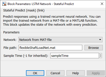
Export the network to Simulink using exportNetworkToSimulink.

Name the model "lstm_model".
To ensure that the Simulink model has its own copy of the network, save the network in the model workspace.
Use the same sample time as for the original model.

exportNetworkToSimulink(net, ...
    ModelName="lstm_model", ...
    SaveNetworkInModelWorkspace=true, ...
    SampleTime=string(sampleTime));

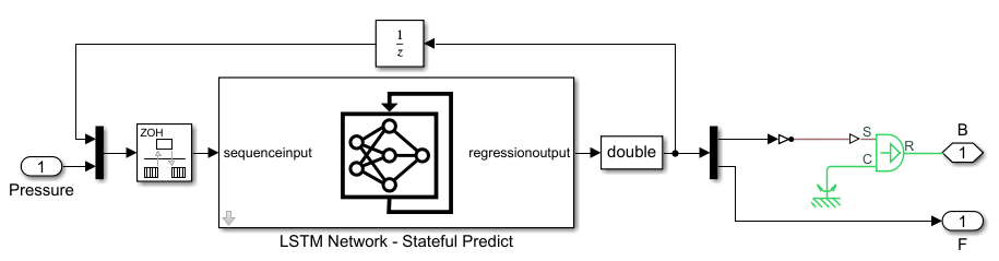
View the subsystem of the model. The subsystem represents the neural network as a model of deep learning layer blocks.

Create the LSTM-ROM component. Create a Simulink component that outputs the predicted B and F signals of the load shaft using the exported model as a subsystem. The model uses the predictions for the next time step through a feedback loop.

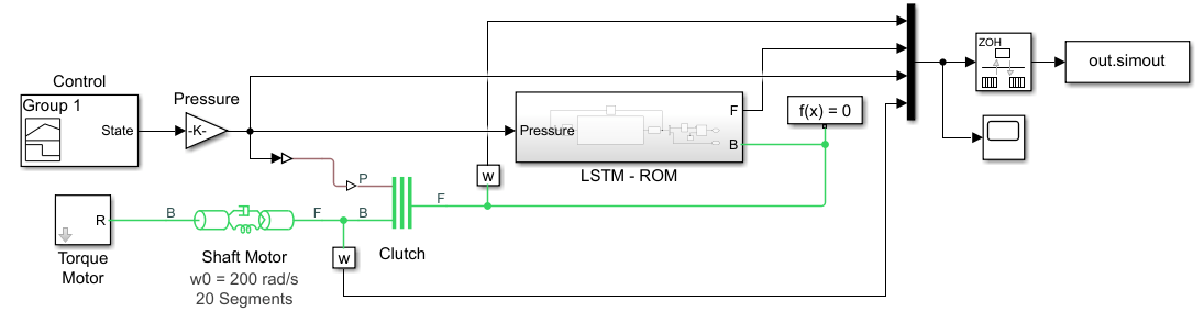
Replace the load shaft in the original Simulink model with the LSTM-ROM subcomponent. The resulting model is saved in ex_sdl_flexible_shaft_lstm. To access this file, open the example as a live script.

Test Model

Evaluate the model accuracy using the held-out test data set.

To test the accuracy of the full model, not just the LSTM network, compare the outputs with the simulated F signals of the motor shaft generated by the original Simulink model.

Extract the targets from the test data. The test targets are simulated F signals of the motor shaft using the original model, shifted by one time step.

numObservationsTest = numel(dataTest);

outputStatesTest = 4;

for i = 1:numObservationsTest
    TTest{i} = dataTest{i}(2:end, outputStatesTest);
end

For each of the maximum pressure values of the test data set, run the simulation and save the simulated F signals of the motor shaft in the cell array YTest.

errs = [];
for i = 1:numObservationsTest
    maxPressure = maxPressuresTest(i);
    simout = sim("ex_sdl_flexible_shaft_lstm");

    YTest{i} = simout.simout.Data(1:end-1,4);
end

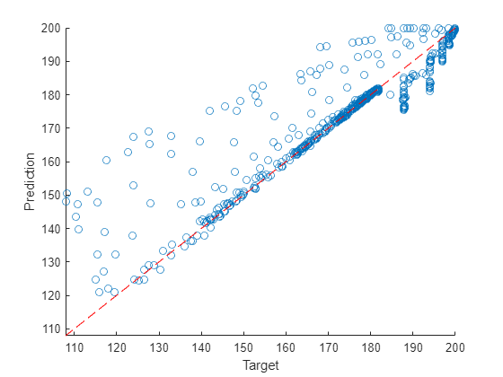
Visualize the time step predictions in a scatter plot.

figure
x = cat(1,TTest{:});
y = cat(1,YTest{:});
scatter(x,y)
xlabel("Target")
ylabel("Prediction")

m = min([x y],[],"all");
M = max([x y],[],"all");
xlim([m M])
ylim([m M])

hold on
plot([m M],[m M],"r--")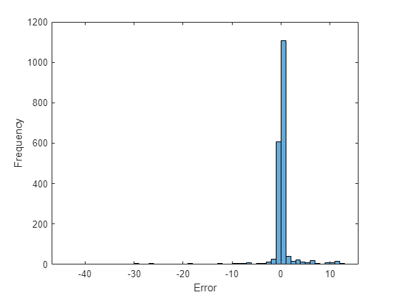

Visualize the prediction errors in a histogram.

figure
histogram([TTest{:}] - [YTest{:}])
xlabel("Error")
ylabel("Frequency")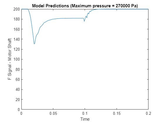

Values close to zero indicate accurate predictions.

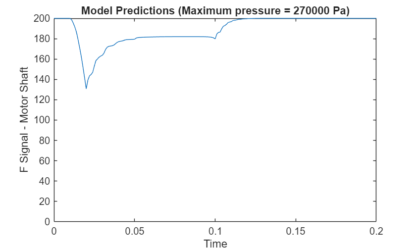
Simulate Using New Data

Run the model with a previously unseen maximum pressure value of $2.7 \times 1 0^{5}$ Pa.

maxPressure = 2.7e5;
simout = sim("ex_sdl_flexible_shaft_lstm");
Y = simout.simout.Data(:,4)';

Visualize the predicted F signal in a plot.

figure
plot(simout.simout.Time, Y)
ylim([0 inf])
xlabel("Time")
ylabel("F Signal - Motor Shaft")
title("Model Predictions (Maximum pressure = " + maxPressure + " Pa)")