Simulate Calorie Burn Using Neural Network in Simulink

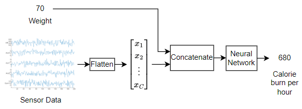
This example shows how to include a simple fully connected neural network in a Simulink® model that predicts calorie burn when given five time steps of sensor readings from a smart watch.

Many neural networks treat time series data differently from other types of data. For example, long short-term memory (LSTM) networks iterate over the time dimension and update a recurrent state, and 1-D convolutional neural networks convolve over the time dimension. Instead, this example uses a simple fully connected neural network that treats the elements in the time dimension as independent features.

This example uses a fully connected neural network that uses flattened time series data. The model takes sequence data represented by (numTimeSteps*numChannels+1)-by-1 vectors, where numTimeSteps is the number of time steps, numChannels is the number of channels, and the +1 corresponds to the additional input channel that takes the weight of the participant.

This type of neural network is small and well suited for Simulink models and deployment to target hardware.

Load Pretrained Network

Load the pretrained neural network in the MAT file CalorieNet.mat.

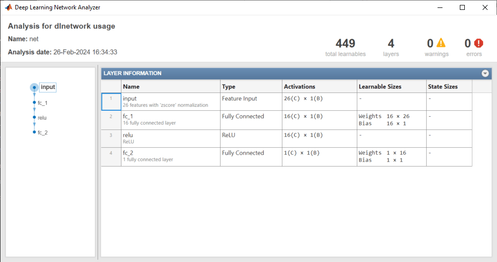
load CalorieNet.mat

View the neural network architecture using the analyzeNetwork function.

• The network expects feature vectors with a size of 26 as input. The first element corresponds to the weight of the participant, the next five elements correspond to the five sensor readings for the first time step. The next five elements correspond to the five sensor readings for the second time step, and so on for the third, fourth, and fifth time steps.

• The network has two fully connected layers.

• The network outputs a single value that represents the estimated calorie burn per hour.

analyzeNetwork(net)

Open Simulink Model

Open the Simulink model.

The model has these data sources:

• The weight of the participant, represented by the Constant block

• The heart rate of the participant, represented as a Ramp block

• Accelerometer and gyro sensor readings, represented by Sine Wave blocks with different amplitudes

The model has these components:

• A Vector Concatenate block that concatenates the sensor data into a five-element vector

• A series of Unit Delay blocks that capture the five time steps of the input data for the neural network

• A Vector Concatenate block that concatenates the weight value and the sensor data into a 26-element vector

• A subsystem that represents the neural network loaded in this example and outputs the estimate of the calorie burn rate

• The calorieNet subsystem, which contains blocks evaluate the neural network used in this example and outputs the estimate of the calorie burn rate

• A Scope block that visualizes the neural network output

open_system("CalorieNet.slx");

Run Simulation

Run the simulation using the sim function.

sim("CalorieNet");

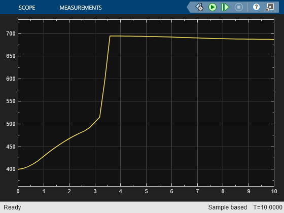
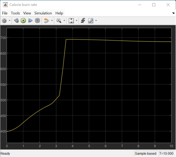
The Scope block shows the calorie burn rate over time. To experiment with the Simulink model, adjust the weight and sensor sources and run the simulation again.