Lowpass Filter Design in MATLAB
This example shows how to design lowpass filters. The example highlights some of the most commonly used command-line tools in the DSP System Toolbox™. For more design options, see Design Lowpass FIR Filters.
Introduction
When designing a lowpass filter, the first choice you make is whether to design an FIR or IIR filter. You generally choose FIR filters when a linear phase response is important. FIR filters also tend to be preferred for fixed-point implementations because they are typically more robust to quantization effects. FIR filters are also used in many high-speed implementations such as FPGAs or ASICs because they are suitable for pipelining. IIR filters (in particular biquad filters) are used in applications (such as audio signal processing) where phase linearity is not a concern. IIR filters are generally computationally more efficient in the sense that they can meet the design specifications with fewer coefficients than FIR filters. IIR filters also tend to have a shorter transient response and a smaller group delay. However, the use of minimum-phase and multirate designs can result in FIR filters comparable to IIR filters in terms of group delay and computational efficiency.
FIR Lowpass Designs - Specifying the Filter Order
There are many practical situations in which you must specify the filter order. One such case is if you are targeting hardware which has constrained the filter order to a specific number. Another common scenario is when you have computed the available computational budget (MIPS) for your implementation and this affords you a limited filter order. FIR design functions in the Signal Processing Toolbox (including fir1, firpm, and firls) are all capable of designing lowpass filters with a specified order. In the DSP System Toolbox, the preferred function for lowpass FIR filter design with a specified order is firceqrip. This function designs optimal equiripple lowpass/highpass FIR filters with specified passband/stopband ripple values and with a specified passband-edge frequency. The stopband-edge frequency is determined as a result of the design.
Design a lowpass FIR filter for data sampled at 48 kHz. The passband-edge frequency is 8 kHz. The passband ripple is 0.01 dB and the stopband attenuation is 80 dB. Constrain the filter order to 120.
N = 120;
Fs = 48e3;
Fp = 8e3;
Ap = 0.01;
Ast = 80;
Obtain the maximum deviation for the passband and stopband ripples in linear units.
Rp = (10^(Ap/20) - 1)/(10^(Ap/20) + 1);
Rst = 10^(-Ast/20);
Design the filter using firceqrip and view the magnitude frequency response.
NUM = firceqrip(N,Fp/(Fs/2),[Rp Rst],"passedge");
hFiltAnalyzer = filterAnalyzer(NUM,SampleRates=Fs,FilterNames="Num_120")
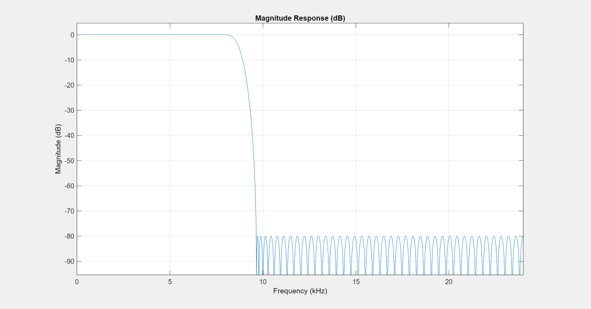
hFiltAnalyzer =
  filterAnalyzer with no properties.
The resulting stopband-edge frequency is about 9.64 kHz.
Minimum-Order Designs
Another design function for optimal equiripple filters is firgr. firgr can design a filter that meets passband/stopband ripple constraints as well as a specified transition width with the smallest possible filter order. For example, if the stopband-edge frequency is specified as 10 kHz, the resulting filter has an order of 100 rather than the 120th-order filter designed with firceqrip. The smaller filter order results from the larger transition band.
Specify the stopband-edge frequency of 10 kHz. Obtain a minimum-order FIR filter with a passband ripple of 0.01 dB and 80 dB of stopband attenuation.
Fst = 10e3;
NumMin = firgr("minorder",[0 Fp/(Fs/2) Fst/(Fs/2) 1],...
    [1 1 0 0],[Rp,Rst]);
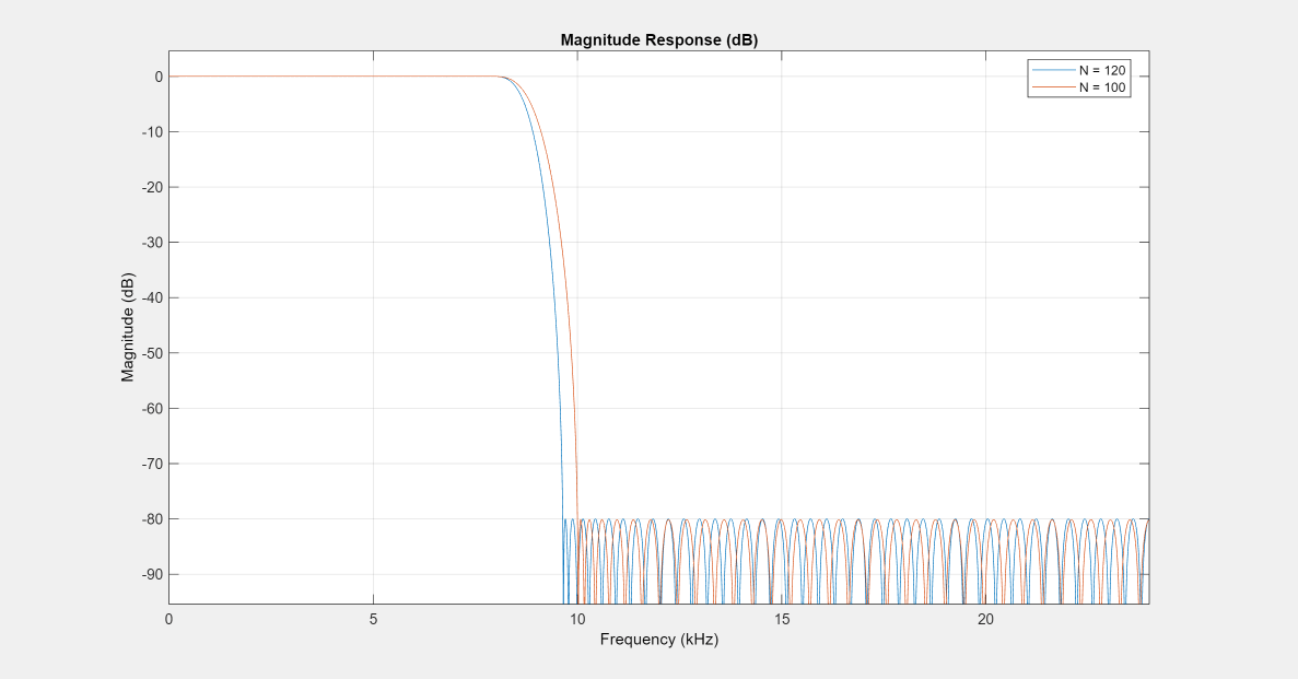
Plot the magnitude frequency responses for the minimum-order FIR filter obtained with firgr and the 120th-order filter designed with firceqrip. The minimum-order design results in a filter with order 100. The transition region of the 120th-order filter is, as expected, narrower than that of the filter with order 100.
hFiltAnalyzer.addFilters(NumMin,FilterNames="Num_minorder");
hFiltAnalyzer.setLegendStrings(["N = 120" "N = 100"]);
Filtering Data
To apply the filter to data, you can use the filter command or you can use dsp.FIRFilter. dsp.FIRFilter has the advantage of managing state when executed in a loop. dsp.FIRFilter also has fixed-point capabilities and supports C code generation, HDL code generation, and optimized code generation for ARM® Cortex® M and ARM Cortex A.
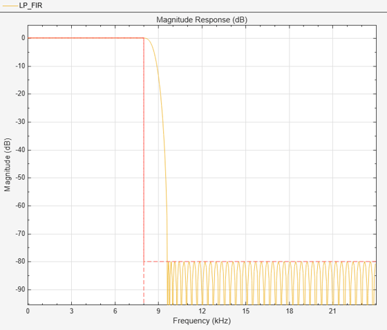
Filter 10 seconds of white noise with zero mean and unit standard deviation in frames of 256 samples with the 120th-order FIR lowpass filter. View the result on a spectrum analyzer.
LP_FIR = dsp.FIRFilter(Numerator=NUM);
SA_FIR = spectrumAnalyzer(SampleRate=Fs,PlotAsTwoSidedSpectrum=false);
tic
while toc < 10
    x = randn(256,1);
    y = LP_FIR(x);
    step(SA_FIR,y);
end
release(SA_FIR)
Using dsp.LowpassFilter
dsp.LowpassFilter is an alternative to using firceqrip and firgr in conjunction with dsp.FIRFilter. Basically, dsp.LowpassFilter condenses the two step process into one. dsp.LowpassFilter provides the same advantages that dsp.FIRFilter provides in terms of fixed-point support, C code generation support, HDL code generation support, and ARM Cortex code generation support.
Design a lowpass FIR filter for data sampled at 48 kHz. The passband-edge frequency is 8 kHz. The passband ripple is 0.01 dB and the stopband attenuation is 80 dB. Constrain the filter order to 120. Create a dsp.FIRFilter based on your specifications.
LP_FIR = dsp.LowpassFilter(SampleRate=Fs,...
    DesignForMinimumOrder=false,FilterOrder=N,...
    PassbandFrequency=Fp,...
    PassbandRipple=Ap,StopbandAttenuation=Ast);
The coefficients in LP_FIR are identical to the coefficients in NUM.
NUM_LP = tf(LP_FIR);
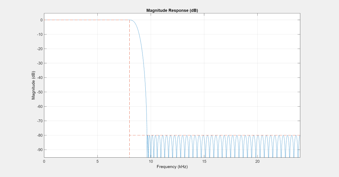
You can use LP_FIR to filter data directly, as shown in the preceding example. You can also analyze the filter using filterAnalyzer or measure the response using measure.
hFiltAnalyzer.addDisplays(1);
hFiltAnalyzer.addFilters(LP_FIR);
measure(LP_FIR)
ans =
Sample Rate      : 48 kHz
Passband Edge    : 8 kHz
3-dB Point       : 8.5843 kHz
6-dB Point       : 8.7553 kHz
Stopband Edge    : 9.64 kHz
Passband Ripple  : 0.01 dB
Stopband Atten.  : 79.9981 dB
Transition Width : 1.64 kHz
Minimum-Order Designs with dsp.LowpassFilter
You can use dsp.LowpassFilter to design minimum-order filters and use measure to verify that the design meets the prescribed specifications. The order of the filter is again 100.
LP_FIR_minOrd = dsp.LowpassFilter(SampleRate=Fs,...
    DesignForMinimumOrder=true,...
    PassbandFrequency=Fp,...
    StopbandFrequency=Fst,...
    PassbandRipple=Ap,...
    StopbandAttenuation=Ast);
measure(LP_FIR_minOrd)
ans =
Sample Rate      : 48 kHz
Passband Edge    : 8 kHz
3-dB Point       : 8.7117 kHz
6-dB Point       : 8.9199 kHz
Stopband Edge    : 10 kHz
Passband Ripple  : 0.0099997 dB
Stopband Atten.  : 80 dB
Transition Width : 2 kHz
Nlp = order(LP_FIR_minOrd)
Nlp =
100
Designing IIR Filters
Elliptic filters are the IIR counterpart to optimal equiripple FIR filters. Accordingly, you can use the same specifications to design elliptic filters. The filter order you obtain for an IIR filter is much smaller than the order of the corresponding FIR filter.
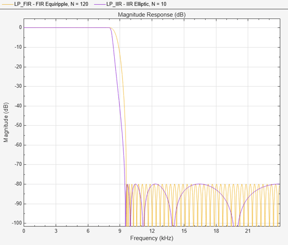
Design an elliptic filter with the same sampling frequency, cutoff frequency, passband-ripple constraint, and stopband attenuation as the 120th-order FIR filter. Reduce the filter order for the elliptic filter to 10.
N = 10;
LP_IIR = dsp.LowpassFilter(SampleRate=Fs,...
    FilterType="IIR",...
    DesignForMinimumOrder=false,...
    FilterOrder=N,...
    PassbandFrequency=Fp,...
    PassbandRipple=Ap,...
    StopbandAttenuation=Ast);
Compare the FIR and IIR designs. Compute the cost of the two implementations.
hFiltAnalyzer.addFilters(LP_IIR);
hFiltAnalyzer.setLegendStrings(["FIR Equiripple, N = 120" "IIR Elliptic, N = 10"])
cost_FIR = cost(LP_FIR)
cost_FIR = struct with fields:
                  NumCoefficients: 121
                        NumStates: 120
    MultiplicationsPerInputSample: 121
          AdditionsPerInputSample: 120
cost_IIR = cost(LP_IIR)
cost_IIR = struct with fields:
                  NumCoefficients: 25
                        NumStates: 20
    MultiplicationsPerInputSample: 25
          AdditionsPerInputSample: 20
The FIR and IIR filters have similar magnitude responses. The cost of the IIR filter is about 1/6 the cost of the FIR filter.
Running the IIR Filters
The IIR filter is designed as a biquad filter. To apply the filter to data, use the same commands as in the FIR case.
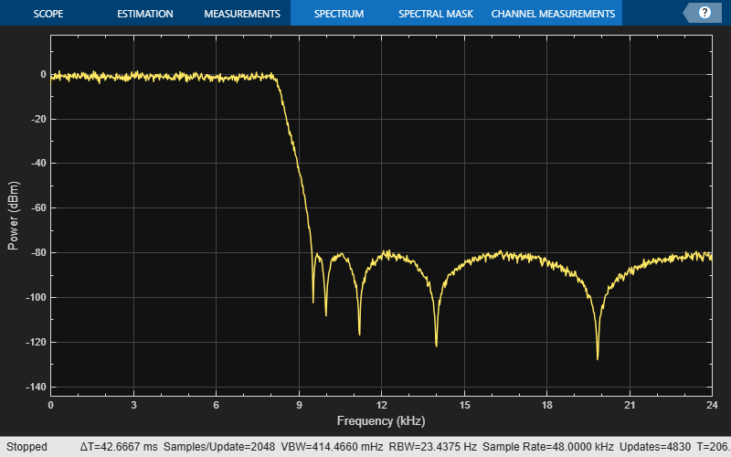
Filter 10 seconds of white Gaussian noise with zero mean and unit standard deviation in frames of 256 samples with the 10th-order IIR lowpass filter. View the result on a spectrum analyzer.
SA_IIR = spectrumAnalyzer(SampleRate=Fs,PlotAsTwoSidedSpectrum=false);
tic
while toc < 10
    x = randn(256,1);
    y = LP_IIR(x);
    SA_IIR(y);
end
release(SA_IIR)
Variable Bandwidth FIR and IIR Filters
You can also design filters that allow you to change the cutoff frequency at run-time. dsp.VariableBandwidthFIRFilter and dsp.VariableBandwidthIIRFilter can be used for such cases.