simsmooth
Bayesian nonlinear non-Gaussian state-space model simulation smoother
Since R2024a
Syntax
Description
simsmooth provides random paths of states drawn from the
posterior smoothed state distribution, which is the distribution of the states conditioned on
model parameters Θ and the full-sample response data, of a Bayesian nonlinear non-Gaussian
state-space model (bnlssm).
To draw state paths from the posterior smoothed state distribution,
simsmooth uses the nonlinear forward-filtering,
backward-sampling method (FFBS), in which it implements sequential Monte Carlo
(SMC) to perform forward filtering, and then it resamples and reweights
particles (weighted random samples) generated by SMC to perform
backward sampling.
X = simsmooth(Mdl,Y,params)simsmooth uses
FFBS to obtain the random path from the posterior smoothed state distribution.
simsmooth evaluates the parameter map
Mdl.ParamMap by using the input vector of parameter values.
X = simsmooth(Mdl,Y,params,Name=Value)simsmooth(Mdl,Y,params,NumPaths=1e4,Resample="residual") specifies
generating 1e4 random paths and to resample residuals.
[
additionally returns the following quantities using any of the input-argument combinations
in the previous syntaxes:X,OutputFilter,x0] = simsmooth(___)
OutputFilter— SMC forward filtering results by sampling time containing the following quantities:Approximate loglikelihood values associated with the input data, input parameters, particles, and posterior state filtering distribution
Filter estimate of state-distribution means
Filter estimate of state-distribution covariance
State particles and corresponding weights that approximate the filtering distribution
Effective sample size
Flags indicating which data the software used to filter
Flags indicating resampling
x0— Simulation-smoothed initial state, computed only when you request this output
Examples
This example draws a random path from the approximate posterior smoothed state distribution of the Bayesian nonlinear state-space model in equation. The state-space model contains two independent, stationary, autoregressive states each with a model constant. The observations are a nonlinear function of the states with Gaussian noise. The prior distribution of the parameters is flat. Symbolically, the system of equations is
and are the unconditional means of the corresponding states. The initial distribution moments of each state are their unconditional mean and covariance.
Create a Bayesian nonlinear state-space model characterized by the system. The observation equation is in equation form, that is, the function composing the states is nonlinear and the innovation series is additive, linear, and Gaussian. The Local Functions section contains two functions required to specify the Bayesian nonlinear state-space model: the state-space model parameter mapping function and the prior distribution of the parameters. You can use the functions only within this script.
Mdl = bnlssm(@paramMap,@priorDistribution)
Mdl =
  bnlssm with properties:

             ParamMap: @paramMap
    ParamDistribution: @priorDistribution
      ObservationForm: "equation"
           Multipoint: [1×0 string]
      ParticleOptions: [1×1 particleoptions]
Mdl is a bnlssm model specifying the state-space model structure and prior distribution of the state-space model parameters. Because Mdl contains unknown values, it serves as a template for posterior analysis with observations.
Simulate a series of 100 observations from the following stationary 2-D VAR process.
where the disturbance series are standard Gaussian random variables.
rng(1,"twister")    % For reproducibility
T = 100;
thetatrue = [0.9; 1; -0.75; -1; 0.3; 0.2; 0.1];
MdlSim = varm(AR={diag(thetatrue([1 3]))},Covariance=diag(thetatrue(5:6).^2), ...
    Constant=thetatrue([2 4]));
XSim = simulate(MdlSim,T);
Compose simulated observations using the following equation.
where the innovation series is a standard Gaussian random variable.
ysim = log(sum(exp(XSim - mean(XSim)),2)) + thetatrue(7)*randn(T,1);
To draw from the approximate posterior smoothed state distribution, the simsmooth function requires response data and a model with known state-space model parameters. Choose a random set with the following constraints:
and are within the unit circle. Use to generate values.
and are real numbers. Use the distribution to generate values.
, , and are positive real numbers. Use the distribution to generate values.
theta13 = (-1+(1-(-1)).*rand(2,1));
theta24 = 3*randn(2,1);
theta567 = chi2rnd(1,3,1);
theta = [theta13(1); theta24(1); theta13(2); theta24(2); theta567];
Draw a random path from the approximate smoothed state posterior distribution by passing the Bayesian nonlinear model, simulated data, and parameter values to simsmooth.
SmoothX = simsmooth(Mdl,ysim,theta);
size(SmoothX)
ans = 1×2

   100     4
SmoothX is a 100-by-4 matrix containing one path drawn from the approximate posterior smoothed state distribution, with rows corresponding to periods in the sample and columns corresponding to the state variables. The simsmooth function uses the FFBS method (SMC and a bootstrap to resample particles and weights) to obtain draws from the posterior smoothed state distribution.
Draw another path, but specify used to simulate the data.
SmoothXSim = simsmooth(Mdl,ysim,thetatrue);
Plot the two paths with the true state values.
figure
tiledlayout(2,1)
nexttile
plot([SmoothX(:,1) SmoothXSim(:,1) XSim(:,1)])
title("x_{t,1}")
legend("Smoothed State, random \theta","Smoothed State, true \theta","XSim")
nexttile
plot([SmoothX(:,3) SmoothXSim(:,3) XSim(:,2)])
title("x_{t,3}")
legend("Smoothed State, random \theta","Smoothed State, true \theta","XSim")
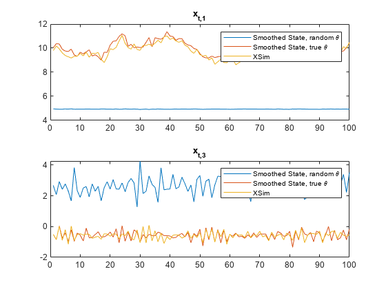
The paths using the true value of and the simulated state paths are close. The paths generated from the random value of is far from the simulated state paths.
Local Functions
These functions specify the state-space model parameter mappings, in equation form, and log prior distribution of the parameters.
function [A,B,C,D,Mean0,Cov0,StateType] = paramMap(theta)
    A = @(x)blkdiag([theta(1) theta(2); 0 1],[theta(3) theta(4); 0 1])*x;
    B = [theta(5) 0; 0 0; 0 theta(6); 0 0];
    C = @(x)log(exp(x(1)-theta(2)/(1-theta(1))) + ...
        exp(x(3)-theta(4)/(1-theta(3))));
    D = theta(7);
    Mean0 = [theta(2)/(1-theta(1)); 1; theta(4)/(1-theta(3)); 1];
    Cov0 = diag([theta(5)^2/(1-theta(1)^2) 0 theta(6)^2/(1-theta(3)^2) 0]);
    StateType = [0; 1; 0; 1];     % Stationary state and constant 1 processes
end

function logprior = priorDistribution(theta)
    paramconstraints = [(abs(theta([1 3])) >= 1); (theta(5:7) <= 0)];
    if(sum(paramconstraints))
        logprior = -Inf;
    else
        logprior = 0;   % Prior density is proportional to 1 for all values
                        % in the parameter space.
    end
end
This example shows how to draw from the posterior distribution of smoothed states and model parameters by using a Gibbs sampler. Consider this nonlinear state-space model
where the parameters in have the following priors:
, that is, a truncated normal distribution with .
, that is, an inverse gamma distribution with shape and scale .
, that is, a gamma distribution with shape and scale .
Simulate Series
Consider this data-generating process (DGP).
where the series is a standard Gaussian series of random variables.
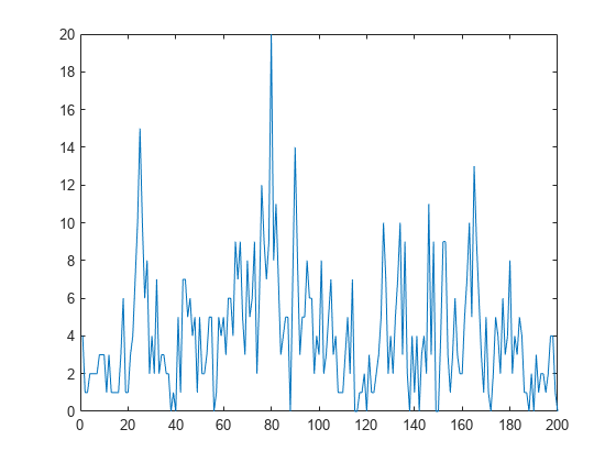
Simulate a series of 200 observations from the process.
rng(500,"twister")    % For reproducibility
T = 200;
thetaDGP = [0.7; 0.2; 3];

numparams = numel(thetaDGP);

MdlXSim = arima(AR=thetaDGP(1),Variance=thetaDGP(2), ...
    Constant=0);
xsim = simulate(MdlXSim,T);
y = random("poisson",thetaDGP(3)*exp(xsim));

figure
plot(y)
Create Bayesian Nonlinear Model
The Local Functions section contains the functions paramMap and logPrior required to specify the Bayesian nonlinear state-space model. The paramMap function specifies the state-space model structure and initial state moments. The priorDistribution function returns the log of the joint prior distribution of the state-space model parameters. You can use the functions only within this script.
Create a Bayesian nonlinear state-space model for the DGP. Indicate that the state-space model observation equation is expressed as a distribution. To speed up computations, the arguments A and LogY of the paramMap function are written to enable simultaneous evaluation of the transition and observation densities of multiple particles. Specify this characteristic by using the Multipoint name-value argument.
Mdl = bnlssm(@paramMap,@priorDistribution,ObservationForm="distribution", ...
    Multipoint=["A" "LogY"]);
Perform Gibbs Sampling
A Gibbs sampler is an Markov chain Monte Carlo method for drawing a sample from the joint posterior distribution of parameters. It successively draws from the full conditional distributions of the states and model parameters, one at a time; results of previous draws are substituted, which enables the Markov chains to explore the parameter space.
The full conditional distribution of the states is the posterior of the smoothed state distribution, which simsmooth computes. The remaining full conditionals are:
, where and.
, where and .
, where and .
You can view the joint posterior distribution as the semiconjugate Bayesian linear regression model , where the response series , predictor series , and the error series . If you view the problem this way, you can speed up sampler. During sampling, you can reject any draws outside its support.
The Local Functions section contains the following functions:
phiFC— Draws fromsigma2FC— Draws fromlambdaFC— Draws from
Conduct the Gibbs sampler. Draw a sample of 2000 from the full conditional distributions. Draw 1500 particles for each call of simsmooth. Perform rejection sampling at a maximum of 50 iterations. This example chooses the initial conditions arbitrarily.
nGibbs = 2000;
Gibbs = zeros(T+numparams,nGibbs); % Preallocate for state and parameter draws
numparticles = 1500;
maxiterations = 50;

% Initial values
% theta
theta0 = [0.5; 0.1; 2];

% pi(phi,sigma2) hyperparameters
m0 = 0;
v02 = 1;
a0 = 1;
b0 = 1;
MdlBLM = semiconjugateblm(1,Intercept=0,Mu=m0,V=v02, ...
    A=a0,B=b0);

% lambda hyperparameters
alpha0 = 3;
beta0 = 1;

hyperparams = [m0 v02 a0 b0 alpha0 beta0];

% Prepare wait bar dialog box
wb = waitbar(0,"1",Name="Running Gibbs Sampler ...", ...
    CreateCancelBtn="setappdata(gcbf,Canceling=true)");
setappdata(wb,Canceling=false);

% Gibbs sampler
theta = theta0;
for j = 1:nGibbs
    % Press Cancel in the dialog to break.
    if getappdata(wb,"Canceling")
        fprintf("Gibbs sampler canceled")
        break
    end
    waitbar(j/nGibbs,wb,sprintf("Draw %d of %d",j,nGibbs));
    Gibbs(1:T,j) = simsmooth(Mdl,y,theta,NumParticles=numparticles, ...
        MaxIterations=maxiterations);
    [Gibbs(T+1,j),Gibbs(T+2,j)] = blmFC(Gibbs(1:T,j),MdlBLM,theta);
    Gibbs(T+3,j) = lambdaFC(Gibbs(1:T,j),y,hyperparams);
    theta = Gibbs(T+(1:3),j);
end
delete(wb)
Describe
To reduce the influence of initial conditions on the sample, remove the first 50 draws from the Gibbs sample. To reduce the influence of serial correlation in the sample, thin the sample by keeping every fourth draw.
burnin = 50;
thin = 4;
pphi = Gibbs(T+1,burnin:thin:end);
psigma2 = Gibbs(T+2,burnin:thin:end);
plambda = Gibbs(T+3,burnin:thin:end);
Plot trace plots of the Gibbs sampler.
figure
h = tiledlayout(3,1);
nexttile
plot(pphi)
title("\pi(\phi|y)")
nexttile
plot(psigma2)
title("\pi(\sigma^2|y)")
nexttile
plot(plambda)
title("\pi(\lambda|y)")
title(h,"Trace Plots")
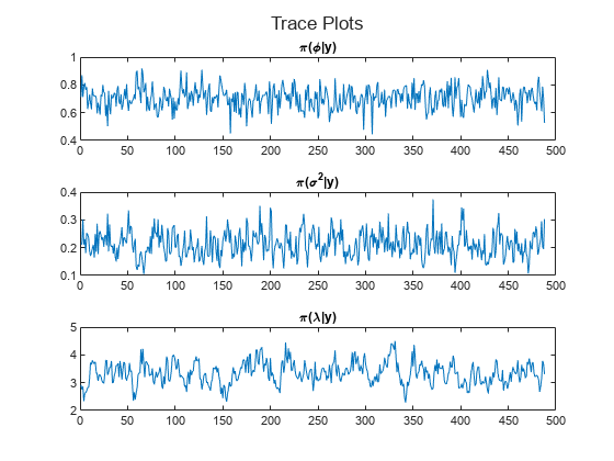
The trace plots show that the Markov chains are mixing adequately.
Summarize the posterior distributions by computing sample medians and 95% percentile intervals of the processed posterior draws. Plot histograms of the posterior distributions of the model parameters.
mphi = median(pphi);
ciphi = quantile(pphi,[0.025 0.975]);
msigma2 = median(psigma2);
cisigma2 = quantile(psigma2,[0.025 0.975]);
mlambda = median(plambda);
cilambda = quantile(plambda,[0.025 0.975]);

figure
h = tiledlayout(3,1);
nexttile
histogram(pphi)
title(sprintf("\\pi(\\phi|y), median=%.3f, ci=(%.3f, %.3f)",mphi,ciphi))
nexttile
histogram(psigma2)
title(sprintf("\\pi(\\sigma^2|y), median=%.3f, ci=(%.3f, %.3f)",msigma2,cisigma2))
nexttile
histogram(plambda)
title(sprintf("\\pi(\\lambda|y), median=%.3f, ci=(%.3f, %.3f)",mlambda,cilambda))
title(h,"Posterior Histograms")
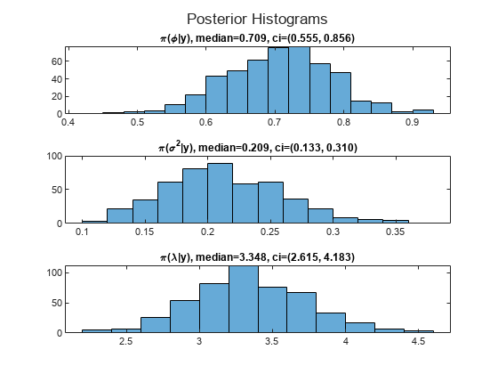
The posterior medians are close to their DGP counterparts.
Local Functions
These functions specify the state-space model parameter mappings, in distribution form, the log prior distribution of the parameters, and random draws from full conditional distribution of each parameter.
function [A,B,LogY,Mean0,Cov0,StateType] = paramMap(theta)
    A = theta(1);
    B = sqrt(theta(2));
    LogY = @(y,x)y.*x - exp(x).*theta(3);
    Mean0 = 0;
    Cov0 = 2;
    StateType = 0;     % Stationary state process
end

function logprior = priorDistribution(theta,hyperparams)
    % Prior of phi
    m0 = hyperparams(1);
    v20 = hyperparams(2);
    pphi = makedist("normal",mu=m0,sigma=sqrt(v20));
    pphi = truncate(pphi,-1,1);
    lpphi = log(pdf(pphi,theta(1)));

    % Prior of sigma2
    a0 = hyperparams(3);
    b0 = hyperparams(4);
    lpsigma2 = -a0*log(b0) - log(gamma(a0)) + (-a0-1)*log(theta(2)) - ...
        1./(b0*theta(2));

    % Prior of lambda
    alpha0 = hyperparams(5);
    beta0 = hyperparams(6);
    plambda = makedist("gamma",alpha0,beta0);
    lplambda = log(pdf(plambda,theta(3)));

    logprior = lpphi + lpsigma2 + lplambda;
end

function [phi,sigma2] = blmFC(x,mdl,theta)
    % Reject sampled phi when it is outside the unit circle
    while true
        phi = simulate(mdl,x(1:end-1),x(2:end),Sigma2=theta(2));
        if abs(phi) < 1
            break
        end
    end
    [~,sigma2] = simulate(mdl,x(1:(end-1)),x(2:end),Beta=theta(1));
end

function [lambda,alpha,beta] = lambdaFC(x,y,hyperparams)
   alpha0 = hyperparams(5);
   beta0 = hyperparams(6);
   alpha = sum(y) + alpha0;
   beta = beta0./(beta0*sum(exp(x))+1);
   lambda = gamrnd(alpha,beta,1);
end
simsmooth runs SMC to forward filter the state-space model, which includes resampling particles. To assess the quality of the sample, including whether any posterior filtered state distribution is close to degenerate, you can monitor these algorithms by returning the third output of smooth.
Consider this nonlinear state-space model.
and are the unconditional means of the corresponding states. The initial distribution moments of each state are their unconditional mean and covariance.
Simulate a series of 100 observations from the following stationary 2-D VAR process.
where the disturbance series and are standard Gaussian random variables.
rng(100,"twister")    % For reproducibility
T = 100;
thetatrue = [0.9; 1; -0.75; -1; 0.3; 0.2; 0.1];
MdlSim = varm(AR={diag(thetatrue([1 3]))},Covariance=diag(thetatrue(5:6).^2), ...
    Constant=thetatrue([2 4]));
XSim = simulate(MdlSim,T);
y = log(sum(exp(XSim - mean(XSim)),2)) + thetatrue(7)*randn(T,1);
Create a Bayesian nonlinear state-space model. The Local Functions section contains the required functions specifying the Bayesian nonlinear state-space model structure and joint prior distribution.
Mdl = bnlssm(@paramMap,@priorDistribution);
Approximate the posterior smoothed state distribution of the state-space model. As in the Draw Path from Posterior Smoothed State Distribution example, choose a random set of initial parameter values. Specify the resampling residuals for the SMC. Return the forward-filtering results and the approximate initial smoothed state .
theta13 = (-1+(1-(-1)).*rand(2,1));
theta24 = 3*randn(2,1);
theta567 = chi2rnd(1,3,1);
theta = [theta13(1); theta24(1); theta13(2); theta24(2); theta567];

[~,OutputFilter,x0] = simsmooth(Mdl,y,theta,Resample="residual");
Output is a 100-by-1 structure array containing several fields, one set of fields for each observation, including:
FilteredStatesCov— Approximate posterior filtered state distribution covariance for the states at each sampling timeDataUsed— Whether the forward-filtering algorithm used an observation for posterior estimationResample— Whether the forward-filtering algorithm resampled the particles associated with an observation
Plot the determinant of the approximate posterior filtered state covariance matrices for states that are not constant.
filteredstatecov = cellfun(@(x)det(x([1 3],[1 3])),{OutputFilter.FilteredStatesCov});

figure
plot(filteredstatecov)
title("Approx. Post. Filtered State Covariances")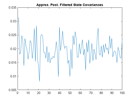
Any covariance determinant that is close to 0 indicates a close-to-degenerate distribution. No covariance determinants in the analysis are close to 0.
Determine whether the forward-filtering algorithm omitted any observations from posterior estimation.
anyObsOmitted = sum([OutputFilter.DataUsed]) ~= T
anyObsOmitted = logical
   0
anyObsOmitted = 0 indicates that the algorithm used all observations.
Determine whether filter resampled any particles associated with observations.
whichResampled = numel(find([OutputFilter.Resampled] == true))
whichResampled =
75
The forward-filtering algorithm resampled particles associated with observations the 75 observations listed in whichResampled.
Local Functions
These functions specify the state-space model parameter mappings, in equation form, and log prior distribution of the parameters.
function [A,B,C,D,Mean0,Cov0,StateType] = paramMap(theta)
    A = @(x)blkdiag([theta(1) theta(2); 0 1],[theta(3) theta(4); 0 1])*x;
    B = [theta(5) 0; 0 0; 0 theta(6); 0 0];
    C = @(x)log(exp(x(1)-theta(2)/(1-theta(1))) + ...
        exp(x(3)-theta(4)/(1-theta(3))));
    D = theta(7);
    Mean0 = [theta(2)/(1-theta(1)); 1; theta(4)/(1-theta(3)); 1];
    Cov0 = diag([theta(5)^2/(1-theta(1)^2) 0 theta(6)^2/(1-theta(3)^2) 0]);
    StateType = [0; 1; 0; 1];     % Stationary state and constant 1 processes
end

function logprior = priorDistribution(theta)
    paramconstraints = [(abs(theta([1 3])) >= 1) (theta(5:7) <= 0)];
    if(sum(paramconstraints))
        logprior = -Inf;
    else
        logprior = 0;   % Prior density is proportional to 1 for all values
                        % in the parameter space.
    end
end
This example compares the performance of several SMC proposal particle resampling methods for obtaining random paths from the posterior smoothed state distribution of a quasi-nonnegative constrained state space model, which models nonnegative state quantities such as interest rates and prices:
and are iid standard Gaussian random variables.
Generate Artificial Data
Consider the following data-generating process (DGP)
Generate a random series of 200 observations from the DGP.
a0 = 0.1;
a1 = 0.95;
b = 1;
d = 0.5;
theta = [a0; a1; b; d];
T = 50;

% Preallocate variables
x = zeros(T,1);
y = zeros(T,1);

rng(0,"twister") % For reproducibility
u = randn(T,1);
e = randn(T,1);

for t = 2:T
    x(t) = max(0,a0 + a1*x(t-1)) + b*u(t);
    y(t) = x(t) + d*e(t);
end
Create Bayesian Nonlinear State-Space Model
The Local Functions section contains two functions required to specify the Bayesian nonlinear state-space model: the state-space model parameter mapping function paramMap and the prior distribution of the parameters priorDistribution. You can use the functions only within this script.
The paramMap function has these qualities:
Functions can simultaneously evaluate the state equation for multiple values of
A. Therefore, you can speed up calculations by specifying theMultipoint="A"option.The observation equation is in equation form, that is, the function composing the states is nonlinear and the innovation series is additive, linear, and Gaussian.
The priorDistribution function specifies a flat prior, which has a density that is proportional to 1 everywhere in the parameter space; it constrains the error standard deviations to be positive.
Create a Bayesian nonlinear state-space model characterized by the system.
Mdl = bnlssm(@paramMap,@priorDistribution,Multipoint="A");Draw Smoothed State Paths from Posterior Using Each Proposal Sampler Method
Obtain a random path from the posterior smoothed state distribution using the joint posterior distribution of the parameters, at a randomly drawn set of values in [0,1], using the bootstrap, optimal, and one-pass unscented particle resampling methods. Specify drawing 5000 particles for SMC.
numParticles = 5000;
smcMethod = ["bootstrap" "optimal" "unscented"];
params = rand(4,1);
for j = 3:-1:1 % Set last element first to preallocate entire cell vector
    xSS{j} = simsmooth(Mdl,y,params,NewSamples=smcMethod(j),NumParticles=numParticles,NumPaths=100);
    XSSStats{j} = quantile(squeeze(xSS{j}),[0.025 0.5 0.975],2);
end
Compare the smoothed state paths from each method with the true values.
figure
tiledlayout(3,1)
for j = 1:3
    nexttile
    h1 = plot([x XSSStats{j}(:,2)]);
    hold on
    h2 = plot(XSSStats{j}(:,[1 3]),"g--");
    hold off
    title("SMC Method: " + upper(smcMethod(j)))
end
legend([h1; h2(1)],["True" "Median" "95% Interval"])
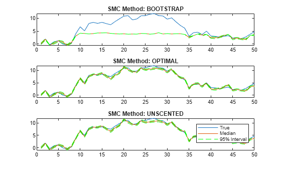
The figure shows that, in this case, the optimal and one-pass unscented methods yield simulated smoothed state estimates closer to the true values than the bootstrap method. For the bootstrap method, simulated smoothed state estimates in periods 10 through 35 level off around 5, while the true values jump as high as 10. The reason is the bootstrap filter updates particles solely by the transition equation—observations do not inform how particles are updated unlike the optimal and unscented methods.
Regardless of method, simsmooth weighs particles by the observation densities. In this example, the observation equation is . For the bootstrap filter, the normally distributed observation innovation, with small loading 0.17, cannot accommodate large jumps, such as from 5 to 10. Consequently, the weights are degenerate: the largest particle takes all the weight, and simsmooth discards the remaining particles during resampling because they have zero weight. The simulated smoothed state estimates level off until period 35 when the observations fall below 5.
Local Functions
These functions specify the state-space model parameter mappings, in equation form, and log prior distribution of the parameters.
function [A,B,C,D,mean0,Cov0] = paramMap(params)
    a0 = params(1);
    a1 = params(2);
    b = params(3);
    d = params(4);
    A = @(x) max(0,a0+a1.*x);
    B = b;
    C = 1;
    D = d;
    mean0 = 0;
    Cov0 = 1;
end

function logprior = priorDistribution(theta)
    paramconstraints = theta(3:4) <= 0; % b and d are greater than 0
    if(sum(paramconstraints))
        logprior = -Inf;
    else
        logprior = 0;   % Prior density is proportional to 1 for all values
                        % in the parameter space.
    end
end
Input Arguments
Name-Value Arguments
Output Arguments
Tips
Smoothing has several advantages over filtering.
The smoothed state estimator is more accurate than the online filter state estimator because it is based on the full-sample data, rather than only observations up to the estimated sampling time.
A stable approximation to the gradient of the loglikelihood function, which is important for numerical optimization, is available from the smoothed state samples of the simulation smoother (finite differences of the approximated loglikelihood computed from the filter state estimates is numerically unstable).
You can use the simulation smoother to perform Bayesian estimation of the nonlinear state-space model via the Metropolis-within-Gibbs sampler.
Unless you set
Cutoff=0,simsmoothresamples particles according to the specified resampling methodResample. Although resampling particles with high weights improves the results of the SMC, you should also allow the sampler traverse the proposal distribution to obtain novel, high-weight particles. To do this, experiment withCutoff.Avoid an arbitrary choice of the initial state distribution.
bnlssmfunctions generate the initial particles from the specified initial state distribution, which impacts the performance of the nonlinear filter. If the initial state specification is bad enough, importance weights concentrate on a small number of particles in the first SMC iteration, which might produce unreasonable filtering results. This vulnerability of the nonlinear model behavior contrasts with the stability of the Kalman filter for the linear model, in which the initial state distribution usually has little impact on the filter because the prior is washed out as it processes data.
Algorithms
simsmooth accommodates missing data by not updating filtered state estimates corresponding to missing observations. In other words, suppose there is a missing observation at period t. Then, the state forecast for period t based on the previous t – 1 observations and filtered state for period t are equivalent.
References
[6] Fernández-Villaverde, Jesús, and Juan F. Rubio-Ramírez. "Estimating Macroeconomic Models: A Likelihood Approach." Review of Economic Studies 70(October 2007): 1059–1087. https://doi.org/10.1111/j.1467-937X.2007.00437.x.