Main Content

cffilter

Christiano-Fitzgerald filter for trend and cyclical components

Since R2023a

Description

The cffilter function applies the Christiano-Fitzgerald filter to separate one or more time series into additive trend and cyclical components. cffilter optionally plots the series and trend component, with cycles removed.

In addition to the Christiano-Fitzgerald filter, Econometrics Toolbox™ supports the Baxter-King (bkfilter), Hamilton (hfilter), and Hodrick-Prescott (hpfilter) filters.

example

[Trend,Cyclical] = cffilter(Y) returns the additive trend Trend and cyclical Cycilcal components from applying the Christiano-Fitzgerald filter [2] to each variable (column) of the input matrix of time series data Y, using the definition of a business cycle in [1] for quarterly data.

example

[TTbl,CTbl] = cffilter(Tbl) returns tables or timetables containing variables for the trend and cyclical components from applying the Christiano-Fitzgerald filter to each variable in an input table or timetable. To select different variables to filter, use the DataVariables name-value argument.

example

[___] = cffilter(___,Name=Value) specifies options using one or more name-value arguments in addition to any of the input argument combinations in previous syntaxes. cffilter returns the output argument combination for the corresponding input arguments. For example, cffilter(Tbl,Symmetric=true,Drift=[false false true],DataVariables=1:3) applies the symmetric Christiano-Fitzgerald filter to the first three variables in the input table Tbl, and removes the linear drift term from the third variable before applying the filter.

example

cffilter(___) plots time series variables in the input data and their respective smoothed trend components (cycles removed), computed by the Christiano-Fitzgerald filter, on the same axes.

cffilter(ax,___) plots on the axes specified by ax instead of the current axes (gca). ax can precede any of the input argument combinations in the previous syntaxes.

example

[___,h] = cffilter(___) plots the specified series and their trend components, and additionally returns handles to plotted graphics objects. Use elements of h to modify properties of the plot after you create it.

Examples

collapse all

Plot the cyclical component of the US post-WWII, seasonally adjusted, quarterly, real gross national product (GNPR).

load Data_GNP
GNPR = Data(:,2);
[trend,cyclical] = cffilter(GNPR);
T = numel(trend)
T = 235

trend and cyclical are 235-by-1 vectors containing the trend and cyclical components, respectively, resulting from applying the asymmetric Christiano-Fitzgerald filter to the series with default upper and lower cutoffs.

plot(dates,cyclical) 
axis tight
ylabel("Real GNP Cyclical Component")

Apply the Christiano-Fitzgerald filter to all variables in input table variables.

Load the Schwert stock data set Data_SchwertStock.mat, which contains monthly returns of the NYSE index from 1871 through 2008 in DataTimeTableMth, among three other variables (for details, enter Description). Remove all missing observations from all series.

load Data_SchwertStock
TTM = rmmissing(DataTimeTableMth);

Aggregate the monthly data in the timetable to quarterly measurements.

TTQ = convert2quarterly(TTM);

Apply the asymmetric Christiano-Fitzgerald filter to all variables in the quarterly timetable. Use the default cutoffs.

[TQTT,CQTT] = cffilter(TTQ);
size(TQTT)
ans = 1×2

   220     4

TQTT and CQTT are 220-by-4 timetables containing the trend and cyclical components, respectively, of the series in TTQ. Variables in the input and output timetables correspond. By default, cffilter filters all variables in the input table or timetable. To select a subset of variables, set the DataVariables option.

To compare outputs between different tabular inputs, apply the Christiano-Fitzgerald filter to all variables in the table of monthly data DataTableMth and the timetable of monthly data TTM.

% Table input of daily data
DTM = rmmissing(DataTableMth);
[TMDT,CMDT] = cffilter(DTM);
size(TMDT)
ans = 1×2

   656     4

tail(TMDT)
                 Return       DivYld       CapGain       CapGainA 
               __________    _________    __________    __________

    May1925      0.082825    0.0030391      0.079846      0.079786
    Jun1925      0.005878    0.0057145    0.00023547    0.00016356
    Jul1925      0.014371    0.0054548     0.0089194     0.0089158
    Aug1925      0.046424    0.0033349      0.043012       0.04309
    Sep1925      0.022868    0.0064024      0.016375      0.016465
    Oct1925      0.079477    0.0058413      0.073612      0.073636
    Nov1925    0.00055416     0.003497    -0.0028871    -0.0029429
    Dec1925      0.050338    0.0068429      0.043564      0.043495
tail(CMDT)
                 Return        DivYld        CapGain       CapGainA  
               __________    ___________    __________    ___________

    May1925     -0.016639    -0.00055599     -0.016143      -0.016083
    Jun1925    -0.0026377    -0.00025619    -0.0024535     -0.0023816
    Jul1925     0.0044847    -0.00024249     0.0047236      0.0047272
    Aug1925     0.0017835    -0.00062296     0.0024837      0.0024064
    Sep1925    -0.0060897     -0.0011003    -0.0048985     -0.0049894
    Oct1925     -0.011281     -0.0012017     -0.010055      -0.010079
    Nov1925    -0.0090187    -0.00068252    -0.0083919     -0.0083361
    Dec1925     -0.000747     0.00024995    -0.0010665    -0.00099695
% Timetable input of daily data
[TMTT,CMTT] = cffilter(TTM);
size(TMTT)
ans = 1×2

   656     4

tail(TMTT)
       Time          Return       DivYld       CapGain       CapGainA 
    ___________    __________    _________    __________    __________

    01-May-1925      0.082825    0.0030391      0.079846      0.079786
    01-Jun-1925      0.005878    0.0057145    0.00023547    0.00016356
    01-Jul-1925      0.014371    0.0054548     0.0089194     0.0089158
    01-Aug-1925      0.046424    0.0033349      0.043012       0.04309
    01-Sep-1925      0.022868    0.0064024      0.016375      0.016465
    01-Oct-1925      0.079477    0.0058413      0.073612      0.073636
    01-Nov-1925    0.00055416     0.003497    -0.0028871    -0.0029429
    01-Dec-1925      0.050338    0.0068429      0.043564      0.043495
tail(CMTT)
       Time          Return        DivYld        CapGain       CapGainA  
    ___________    __________    ___________    __________    ___________

    01-May-1925     -0.016639    -0.00055599     -0.016143      -0.016083
    01-Jun-1925    -0.0026377    -0.00025619    -0.0024535     -0.0023816
    01-Jul-1925     0.0044847    -0.00024249     0.0047236      0.0047272
    01-Aug-1925     0.0017835    -0.00062296     0.0024837      0.0024064
    01-Sep-1925    -0.0060897     -0.0011003    -0.0048985     -0.0049894
    01-Oct-1925     -0.011281     -0.0012017     -0.010055      -0.010079
    01-Nov-1925    -0.0090187    -0.00068252    -0.0083919     -0.0083361
    01-Dec-1925     -0.000747     0.00024995    -0.0010665    -0.00099695

Because the data is disaggregated, the outputs of the daily data have more rows than from the quarterly data. The filter results of the daily inputs are equal among the corresponding outputs, but cffilter returns tables of results, instead of timetables, when you supply data in a table.

Load the Nelson-Plosser macroeconomic data set Data_NelsonPlosser.mat, which contains series measured yearly in the timetable DataTimeTable.
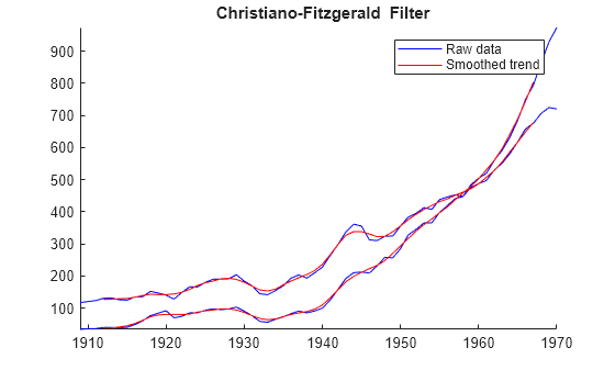
load Data_NelsonPlosser

Apply the asymmetric Christiano-Fitzgerald filter to the real and nominal GNP series, GNPR and GNPN, respectively. Filter out cyclical component frequencies outside the interval [2,8]. Plot the trend component with each series.

figure
cffilter(DataTimeTable,DataVariables=["GNPR" "GNPN"], ...
    LowerCutoff=2,UpperCutoff=8);

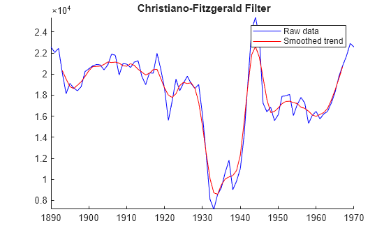
Compare the results of the asymmetric filter with the symmetric filter. in addition to cyclical component cutoffs of 2 and 8, and set the lag length of the symmetric moving average to 3 years.

figure
cffilter(DataTimeTable,DataVariables=["GNPR" "GNPN"], ...
    LowerCutoff=2,UpperCutoff=8,FilterType="symmetric",LagLength=3);

Unlike the asymmetric filter, the first and last LagLength=3 values of the returned components of the symmetric filter are NaN-valued.

Experiment with filter parameter values by adjusting the interactive controls. Because this setup always sets the lag length of the symmetric moving average, cffilter implements the symmetric method only.

varnames = string(DataTimeTable.Properties.VariableNames);
lc = 2; % LowerCutoff
uc = 8; % UpperCutoff
q = 3; % LagLength
tfs = false; % Stationarity
tfd = true; % Drift
vn = varnames(5); % DataVariables

figure
[TTbl,CTbl,h] = cffilter(DataTimeTable,DataVariables=vn, ...
    LowerCutoff=lc,UpperCutoff=uc,LagLength=q,Stationarity=tfs, ...
    Drift=tfd);

Input Arguments

collapse all

Time series data, specified as a numObs-by-numVars numeric matrix. Each column of Y corresponds to a variable, and each row corresponds to an observation.

Data Types: double

Time series data, specified as a table or timetable with numObs rows. Each row of Tbl is an observation.

Specify numVars variables to filter by using the DataVariables argument. The selected variables must be numeric.

Axes on which to plot, specified as an Axes object.

By default, cffilter plots to the current axes (gca).

Note

cffilter removes, from the specified data, all rows containing at least one missing observation, represented by a NaN value.

Name-Value Arguments

Specify optional pairs of arguments as Name1=Value1,...,NameN=ValueN, where Name is the argument name and Value is the corresponding value. Name-value arguments must appear after other arguments, but the order of the pairs does not matter.

Before R2021a, use commas to separate each name and value, and enclose Name in quotes.

Example: cffilter(Tbl,Symmetric=true,Drift=[false false true],DataVariables=1:3) applies the symmetric Christiano-Fitzgerald filter to the first three variables in the input table Tbl, and removes the linear drift term from the third variable before applying the filter.

Lower cutoff period for the cyclical component, in units of data periodicity, specified as a numeric scalar or a length numVars vector with elements greater than or equal to 2.

For a scalar, cffilter uses LowerCutoff for all input series.

For a vector, cffilter applies LowerCutoff(j) to selected j in the input data.

The default is 6, meaning 6 quarters (18 months), which is based on the definition of business cycle in [1].

For more details, see Tips

Example: LowerCutoff=[4 6] applies a lower cutoff of 4 to the first series in the input data and a lower cutoff of 6 to the second series.

Data Types: double

Upper cutoff period for the cyclical component, in units of data periodicity, specified as a numeric scalar or a length numVars vector with elements greater than or equal to the corresponding LowerCutoff for each series.

For a scalar, cffilter uses UpperCutoff for all input series.

For a vector, cffilter applies UpperCutoff(j) to series j in the input data.

The default is 32, meaning 32 quarters (8 years), which is based on the definition of business cycle in [1].

For more details, see Tips

Example: UpperCutoff=[32 36] applies an upper cutoff of 32 to the first series in the input data and an upper cutoff of 36 to the second series.

Data Types: double

Finite-sample approximation of ideal bandpass filter, specified as a value in this table.

ValueDescription
"asymmetric"Asymmetric, time-varying moving average
"symmetric"Symmetric, time-invariant moving average

If you set LagLength, cffilter sets FilterType to "symmetric".

Example: FilterType="symmetric"

Data Types: char | string

Number of consecutive lags of the moving average for the symmetric filter (see FilterType), specified as a positive integer less than (numObs−1)/2 or vector of such positive integers.

For a scalar, cffilter applies LagLength to all input series.

For a vector, cffilter applies LagLength(j) to series j in the input data.

If you specify LagLength, cffilter sets FilterType to "symmetric".

The default is 12, suggested in [2] for quarterly data.

For more details, see Tips

Example: LagLength=[4 8] sets FilterType to "symmetric" and specifies 4 lags for the symmetric moving average of the first series in the input data and 8 for the symmetric moving average of the second series.

Data Types: double

Flag indicating whether input series is stationary, specified as a value or a vector of values in this table.

ValueDescription
falseInput series is a nonstationary random walk.
trueInput series is stationary; cffilter adjusts the filter to use ideal weights at series endpoints.

For more details on the alternatives, see [2].

For a scalar, cffilter applies Stationarity to all input series.

For a vector, cffilter applies Stationarity(j) to series j in the input data.

Example: Stationarity=[true false] specifies that the first input series is stationary and the second input series is nonstationary.

Data Types: logical

Flag indicating drift in the input series, specified as a value in this table.

ValueDescription
falsecffilter does not linear drift from the input series.
truecffilter removes linear drift from the input series before it applies the filter.

For a scalar, cffilter applies Drift to all input series.

For a vector, cffilter applies Drift(j) to series j in the input data.

Example: Drift=[false true] removes the linear drift from only the second input series.

Data Types: logical

Variables in Tbl that cffilter filters, specified as a string vector or cell vector of character vectors containing variable names in Tbl.Properties.VariableNames, or an integer or logical vector representing the indices of names. The selected variables must be numeric.

Example: DataVariables=["GDP" "CPI"]

Example: DataVariables=[true true false false] or DataVariables=[1 2] selects the first and second table variables.

Data Types: double | logical | char | cell | string

Output Arguments

collapse all

Smoothed trend component τt of each series in the data, returned as a numObs-by-numVars numeric matrix. cffilter returns Trend when you supply the input Y.

When cffilter implements the symmetric filter (see FilterType) for a series, the first and last LagLength values are NaN for the corresponding column in Trend.

Cyclical component ct of each series in the data, returned as a numObs-by-numVars numeric matrix. cffilter returns Cyclical when you supply the input Y.

When cffilter implements the symmetric filter (see FilterType) for a series, the first and last LagLength values are NaN for the corresponding column in Cyclical.

Smoothed trend component τt of each specified series, returned as a numObs-by-numVars table or timetable, the same data type as Tbl. cffilter returns TTbl when you supply the input Tbl.

For each selected series and corresponding LagLength, when cffilter implements the symmetric filter (see FilterType) for a series, the first and last LagLength values are NaN in the corresponding variable in TTbl.

Cyclical component ct of each specified series, returned as a numObs-by-numVars table or timetable, the same data type as Tbl. cffilter returns CTbl when you supply the input Tbl.

For each selected series and corresponding LagLength, when cffilter implements the symmetric filter (see FilterType) for a series, the first and last LagLength values are NaN in the corresponding variable in CTbl.

Handles to plotted graphics objects, returned as a vector of graphics objects. cffilter plots the data and trend only when you return no outputs or you return h.

h contains unique plot identifiers, which you can use to query or modify properties of the plot.

More About

collapse all

Christiano-Fitzgerald Filter

The Christiano-Fitzgerald filter separates a time series yt into a trend component τt (Trend and TTbl) and cyclical component ct (Cyclical and CTbl) such that yt = τt + ct.

Depending on the value of the value of the FilterType name-value argument, cffilter implements either an asymmetric, time-varying, or a symmetric, time-invariant moving average as a finite-sample approximation of an ideal bandpass filter [2].

Tips

The definition of a business cycle in [1] suggests values in the table for the cutoff periods LowerCutoff and UpperCutoff, and lag length LagLength that depend on the periodicity of the data.

PeriodicityLowerCutoffUpperCutoffLagLength
Yearly283
Quarterly63212
Monthly189636

In practice, use vectors of cutoff periods and lag lengths to test alternatives. Use the plot produced by cffilter to compare results among settings.

References

[1] Burns, Arthur F., and Wesley C. Mitchell. Measuring Business Cycles. Cambridge, MA: National Bureau of Economic Research, 1946.

[2] Christiano, Lawrence J., and Terry J. Fitzgerald. "The Band Pass Filter." International Economic Review 44 (May 2003): 435–65. https://doi.org/10.1111/1468-2354.t01-1-00076.

Version History

Introduced in R2023a