Main Content

graphplot

Plot Markov chain directed graph

Description

example

graphplot(mc) creates a plot of the directed graph (digraph) of the discrete-time Markov chain mc. Nodes correspond to the states of mc. Directed edges correspond to nonzero transition probabilities in the transition matrix mc.P.

example

graphplot(mc,Name,Value) uses additional options specified by one or more name-value arguments. Options include highlighting transition probabilities, communicating classes, and specifying class properties of recurrence/transience and period. Also, you can plot the condensed digraph instead, with communicating classes as supernodes.

graphplot(ax,___) plots on the axes specified by ax instead of the current axes (gca) using any of the input argument combinations in the previous syntaxes. The option ax can precede any of the input argument combinations in the previous syntaxes.

example

h = graphplot(___) returns the handle to the digraph plot. Use h to modify properties of the plot after you create it.

Examples

collapse all

Consider this theoretical, right-stochastic transition matrix of a stochastic process.

P=[001/21/41/400001/302/300000001/32/3000001/21/2000003/41/41/21/2000001/43/400000].

Create the Markov chain that is characterized by the transition matrix P.

P = [ 0   0  1/2 1/4 1/4  0   0 ;
      0   0  1/3  0  2/3  0   0 ;
      0   0   0   0   0  1/3 2/3;
      0   0   0   0   0  1/2 1/2;
      0   0   0   0   0  3/4 1/4;
     1/2 1/2  0   0   0   0   0 ;
     1/4 3/4  0   0   0   0   0 ];
mc = dtmc(P);

Plot a directed graph of the Markov chain.

figure;
graphplot(mc);

Consider this theoretical, right-stochastic transition matrix of a stochastic process.

P=[0.50.5000.500.5000010010].

Create the Markov chain that is characterized by the transition matrix P. Name the states Regime 1 through Regime 4.

P = [0.5 0.5 0 0; 0.5 0 0.5 0; 0 0 0 1; 0 0 1 0];
mc = dtmc(P,'StateNames',["Regime 1" "Regime 2" "Regime 3" "Regime 4"]);

Plot a directed graph of the Markov chain. Identify the communicating classes in the digraph and color the edges according to the probability of transition.

figure;
graphplot(mc,'ColorNodes',true,'ColorEdges',true)

States 3 and 4 compose a communicating class with period 2. States 1 and 2 are transient.

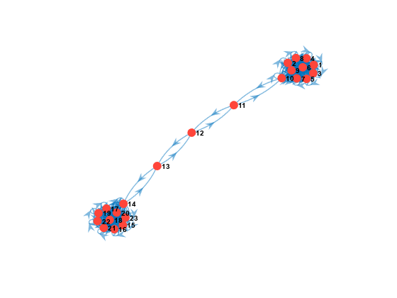
Create a "dumbbell" Markov chain containing 10 states in each "weight" and three states in the "bar."

  • Specify random transition probabilities between states within each weight.

  • If the Markov chain reaches the state in a weight that is closest to the bar, then specify a high probability of transitioning to the bar.

  • Specify uniform transitions between states in the bar.

rng(1); % For reproducibility
w = 10;                              % Dumbbell weights
DBar = [0 1 0; 1 0 1; 0 1 0];        % Dumbbell bar
DB = blkdiag(rand(w),DBar,rand(w));  % Transition matrix

% Connect dumbbell weights and bar
DB(w,w+1) = 1;                       
DB(w+1,w) = 1; 
DB(w+3,w+4) = 1; 
DB(w+4,w+3) = 1;

db = dtmc(DB);

Plot a directed graph of the Markov chain. Return the plot handle.

figure;
h = graphplot(db);

Observe that the state labels are difficult to read. Remove the labels entirely.

h.NodeLabel = {};

Input Arguments

collapse all

Discrete-time Markov chain with NumStates states and transition matrix P, specified as a dtmc object. P must be fully specified (no NaN entries).

Axes on which to plot, specified as an Axes object.

By default, graphplot plots to the current axes (gca).

Name-Value Arguments

Specify optional pairs of arguments as Name1=Value1,...,NameN=ValueN, where Name is the argument name and Value is the corresponding value. Name-value arguments must appear after other arguments, but the order of the pairs does not matter.

Before R2021a, use commas to separate each name and value, and enclose Name in quotes.

Example: 'ColorEdges',true,'ColorNodes',true colors the edges to indicate transition probabilities and colors the nodes based on their communicating class.

Flag for labeling nodes using state names, specified as the comma-separated pair consisting of 'LabelNodes' and a value in this table.

ValueDescription
trueLabel nodes using the names in mc.StateNames.
falseLabel nodes using state numbers.

Example: 'LabelNodes',false

Data Types: logical

Flag for coloring nodes based on communicating class, specified as the comma-separated pair consisting of 'ColorNodes' and a value in this table.

ValueDescription
trueNodes in the same communicating class have the same color. Solid markers represent nodes in recurrent classes, and hollow markers represent nodes in transient classes. The legend contains the periodicity of recurrent classes.
falseAll nodes have the same color.

Example: 'ColorNodes',true

Data Types: logical

Flag for labeling edges with the transition probabilities in the transition matrix mc.P, specified as the comma-separated pair consisting of 'LabelEdges' and a value in this table.

ValueDescription
trueLabel edges with transition probabilities rounded to two decimal places.
falseDo not label edges.

Example: 'LabelEdges',true

Data Types: logical

Flag for coloring edges to indicate transition probabilities, specified as the comma-separated pair consisting of 'ColorEdges' and a value in this table.

ValueDescription
trueColor edges to indicate transition probabilities. Include a color bar, which summarizes the color coding.
falseUse the same color for all edges.

Example: 'ColorEdges',true

Data Types: logical

Flag for condensing the graph, with each communicating class represented by a single supernode, specified as the comma-separated pair consisting of 'Condense' and a value in this table.

ValueDescription
trueNodes are supernodes containing communicating classes. Node labels list the component states of each supernode. An edge from supernode i to supernode j indicates a nonzero probability of transition from some state in supernode i to some state in supernode j. Transition probabilities between supernodes are not well defined, and graphplot disables edge information.
falseNodes are states in mc.

Example: 'Condense',true

Data Types: logical

Output Arguments

collapse all

Handle to the graph plot, returned as a graphics object. h is a unique identifier, which you can use to query or modify properties of the plot.

Tips

  • To produce the directed graph as a MATLAB® digraph object and use additional functions of that object, enter:

    G = digraph(mc.P)

  • For readability, the 'LabelNodes' name-value pair argument allows you to turn off lengthy node labels and replace them with node numbers. To remove node labels completely, set h.NodeLabel = {};.

  • To compute node information on communicating classes and their properties, use classify.

  • To extract a communicating class in the graph, use subchain.

  • The condensed graph is useful for:

    • Identifying transient classes (supernodes with positive outdegree)

    • Identifying recurrent classes (supernodes with zero outdegree)

    • Visualizing the overall structure of unichains (chains with a single recurrent class and any transient classes that transition into it)

References

[1] Gallager, R.G. Stochastic Processes: Theory for Applications. Cambridge, UK: Cambridge University Press, 2013.

[2] Horn, R., and C. R. Johnson. Matrix Analysis. Cambridge, UK: Cambridge University Press, 1985.

[3] Jarvis, J. P., and D. R. Shier. "Graph-Theoretic Analysis of Finite Markov Chains." In Applied Mathematical Modeling: A Multidisciplinary Approach. Boca Raton: CRC Press, 2000.

Version History

Introduced in R2017b