lazy
Adjust Markov chain state inertia
Description
Examples
Consider this three-state transition matrix.
Create the irreducible and periodic Markov chain that is characterized by the transition matrix P.
P = [0 1 0; 0 0 1; 1 0 0];
mc = dtmc(P);
At time t = 1,..., T, mc is forced to move to another state deterministically.
Determine the stationary distribution of the Markov chain and whether it is ergodic.
xFix = asymptotics(mc)
xFix = 1×3

    0.3333    0.3333    0.3333
isergodic(mc)
ans = logical
   0
mc is irreducible and not ergodic. As a result, mc has a stationary distribution, but it is not a limiting distribution for all initial distributions.
Show why xFix is not a limiting distribution for all initial distributions.
x0 = [1 0 0];
x1 = x0*P
x1 = 1×3

     0     1     0
x2 = x1*P
x2 = 1×3

     0     0     1
x3 = x2*P
x3 = 1×3

     1     0     0
sum(x3 == x0) == mc.NumStates
ans = logical
   1
The initial distribution is reached again after several steps, which implies that the subsequent state distributions cycle through the same sets of distributions indefinitely. Therefore, mc does not have a limiting distribution.
Create a lazy version of the Markov chain mc.
lc = lazy(mc)
lc =
  dtmc with properties:

             P: [3×3 double]
    StateNames: ["1"    "2"    "3"]
     NumStates: 3
lc.P
ans = 3×3

    0.5000    0.5000         0
         0    0.5000    0.5000
    0.5000         0    0.5000
lc is a dtmc object. At time t = 1,..., T, lc "flips a fair coin". It remains in its current state if the "coin shows heads" and transitions to another state if the "coin shows tails".
Determine the stationary distribution of the lazy chain and whether it is ergodic.
lcxFix = asymptotics(lc)
lcxFix = 1×3

    0.3333    0.3333    0.3333
isergodic(lc)
ans = logical
   1
lc and mc have the same stationary distributions, but only lc is ergodic. Therefore, the limiting distribution of lc exists and is equal to its stationary distribution.
Consider this theoretical, right-stochastic transition matrix of a stochastic process.
Create the Markov chain that is characterized by the transition matrix P.
P = [ 0   0  1/2 1/4 1/4  0   0 ;
      0   0  1/3  0  2/3  0   0 ;
      0   0   0   0   0  1/3 2/3;
      0   0   0   0   0  1/2 1/2;
      0   0   0   0   0  3/4 1/4;
     1/2 1/2  0   0   0   0   0 ;
     1/4 3/4  0   0   0   0   0 ];
mc = dtmc(P);
Plot the eigenvalues of the transition matrix on the complex plane.
figure;
eigplot(mc);
title('Original Markov Chain')
Three eigenvalues have modulus one, which indicates that the period of mc is three.
Create lazy versions of the Markov chain mc using various inertial weights. Plot the eigenvalues of the lazy chains on separate complex planes.
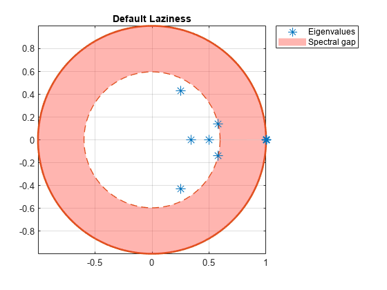
w2 = 0.1;                                 % More active Markov chain
w3 = 0.9;                                 % Lazier Markov chain
w4 = [0.9 0.1 0.25 0.5 0.25 0.001 0.999]; % Laziness differs between states

lc1 = lazy(mc);
lc2 = lazy(mc,w2);
lc3 = lazy(mc,w3);
lc4 = lazy(mc,w4);

figure;
eigplot(lc1);
title('Default Laziness');
figure;
eigplot(lc2);
title('More Active Chain');
figure;
eigplot(lc3);
title('Lazier Chain');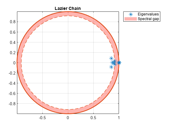
figure;
eigplot(lc4);
title('Differing Laziness Levels');
All lazy chains have only one eigenvalue with modulus one. Therefore, they are aperiodic. The spectral gap (distance between inner and outer circle) determines the mixing time. Observe that all lazy chains take longer to mix than the original Markov chain. Chains with different inertial weights than the default take longer to mix than the default lazy chain.
Input Arguments
Output Arguments
More About
References
[1] Gallager, R.G. Stochastic Processes: Theory for Applications. Cambridge, UK: Cambridge University Press, 2013.
Version History
Introduced in R2017b