Forecast Conditional Mean Model Programmatically

A common objective of time series modeling is to predict responses, or generate forecasts, for a process over a future time period, the forecast horizon. Symbolically, for the observed response series y₁, y₂,...,y_T and a forecast horizon h, the forecasts are y_T+1,y_T+2,…,y_T+h. Forecasts provide insights into the future behavior of a series and aid in decision making. Also, forecasts are often used to assess the predictive performance of several competing models, which complements typical model selection procedures.

You can generate forecasts in a number of ways; this topic shows how to programmatically generate minimum mean squared error (MMSE) forecasts, by using the forecast function, and Monte Carlo forecasts, by using the simulate function, from a conditional mean model of a synthetic series y_t. Although the topic assumes a univariate ARIMA model for y_t, specified as an arima object, the procedure and concepts extend to other models, such as GARCH (garch object) and multivariate VAR (varm object) models.

Regardless of the forecasting method or model, forecasting requires the following inputs:

• Fully-specified model; the model can be calibrated or estimated.

• Forecast horizon, or the number of time steps into the future to generate predictions.

• Presample data to initialize the model for forecasting. Usually, this presample is the response series used to estimate the model.

• Monte Carlo forecasting additionally requires a large number of sample paths.

Generate MMSE and Monte Carlo Forecasts

This example generates and fits synthetic data to an ARIMA(2,1,1) model, and then generates MMSE and Monte Carlo forecasts from the estimated model.

Generate Synthetic Data

Consider this ARIMA model for the data-generating process (DGP).

$$\Delta y_t=1+0.5\Delta y_{t-1}-0.25\Delta y_{t-2}+{\epsilon }_t+0.3{\epsilon }_{t-1},$$

where ${\epsilon }_t$ is an iid series of Gaussian innovations with mean 0 and variance 4.

Create an ARIMA(2,1,1) model for the DGP by using arima. Simulate a path of length $T=100$ from the model.

rng(100,"twister")
DGPMdl = arima(AR={0.5 -0.25},MA=0.3,Constant=1,Variance=4,D=1);
T = 100;
y = simulate(DGPMdl,T);

Choose Model for Series

Typically, the DGP of a series is unknown. This example visually explores the data to determine a suitable model for it, but you can use Econometrics Toolbox™ functions that conduct statistical tests to confirm the conclusions draw by visual inspections (see Model Selection).

Plot the series.

figure
plot(y)
ylabel("y")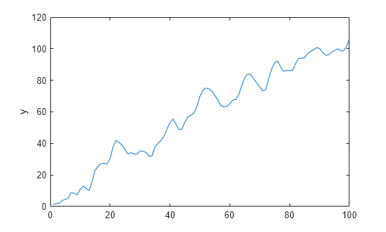

The series appears nonstationary without an exponential trend.

Assume the series is unit root nonstationary. Compute the first difference of the series and plot the result.

dy = diff(y);
figure
plot(dy)
ylabel("\Delta{y}")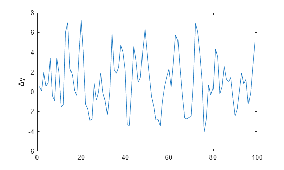

The differenced series appears stationary and homoscedastic.

Plot the ACF and PACF of the differenced series.

figure
autocorr(dy)

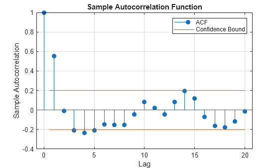
figure
parcorr(dy)

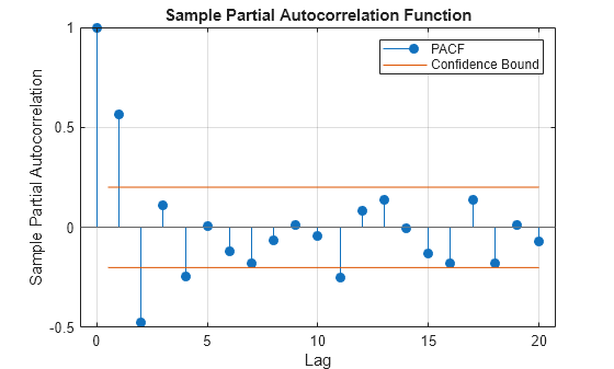
The ACF decays exponentially with a sinusoidal pattern. The PACF cuts off after the second lag. This pattern suggests an ARMA(2,1) model is reasonable for the differenced series or an ARIMA(2,1,1) for the raw series [1].

Fit Model to Data

Create an ARIMA(2,1,1) model template for estimation by using the shorthand syntax of the arima function.

Mdl = arima(2,1,1);

Mdl is a partially specified arima object that specifies the structure of an ARIMA(2,1,1) model. All estimable parameters (the coefficients and variance) correspond to properties of the object and have value NaN.

Fit the model to the data.

EstMdl = estimate(Mdl,y)

 
    ARIMA(2,1,1) Model (Gaussian Distribution):
 
                 Value     StandardError    TStatistic      PValue  
                _______    _____________    __________    __________

    Constant    0.77161       0.31269         2.4677          0.0136
    AR{1}       0.50414       0.17583         2.8673       0.0041403
    AR{2}       -0.2716       0.14808        -1.8342        0.066627
    MA{1}       0.44365       0.18058         2.4568         0.01402
    Variance     3.7067       0.57945          6.397      1.5847e-10

EstMdl = 
  arima with properties:

     Description: "ARIMA(2,1,1) Model (Gaussian Distribution)"
      SeriesName: "Y"
    Distribution: Name = "Gaussian"
               P: 3
               D: 1
               Q: 1
        Constant: 0.771608
              AR: {0.50414 -0.271599} at lags [1 2]
             SAR: {}
              MA: {0.443651} at lag [1]
             SMA: {}
     Seasonality: 0
            Beta: [1×0]
        Variance: 3.70671

EstMdl is a fully specified arima object with the same model structure as Mdl; estimate sets all estimable parameters to the maximum likelihood estimates. The estimates are close to their corresponding true values.

Generate MMSE Forecasts

The forecast functions of Econometrics Toolbox™ univariate and multivariate linear model objects generate analytical MMSE forecasts and standard errors (see MMSE Forecasts and Forecast Mean Squared Error (MSE) and Inferences).

Forecast the estimated ARIMA(2,1,1) model into a 10 step forecast horizon. Return analytical standard errors. Initialize the model for forecasting by setting the presample to the entire series; by default, forecast uses only the required number of observations from the end of the series.

fh = 10;
[fy,fmse] = forecast(EstMdl,fh,Y0=y);

Plot the forecasts and 95% forecast intervals.

alpha = 0.05;
FYCI = fy + norminv(alpha/2)*[1 -1].*sqrt(fmse);
fht = T + (1:fh)';
int = T-50:T;

figure
p1 = plot(int,y(int));
hold on
xline(T,Color=[0.5 0.5 0.5])
p2 = patch([T; fht; flipud(fht); T], [y(end); FYCI(:,2); flipud(FYCI(:,1)); y(end)],"k");
p2.FaceColor = [0.0431 0.1843 0.3608];
p2.EdgeColor = [0.0431 0.1843 0.3608];
p3 = plot([T; fht],[y(end); fy],":",LineWidth=2,Color=[0.1490 0.5490 0.8660]);
hold off
legend([p1 p3 p2],["y" "Forecast" "Confidence Interval"],Location="best")
grid on
title("MMSE Forecasts and Forecast Intervals")

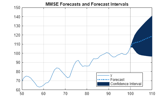
The forecast interval widths widen with increasing steps ahead in the forecast horizon. This is characteristic of forecasts from nonstationary models.

Generate Monte Carlo Forecasts

The simulate functions of Econometrics Toolbox™ model objects draw sample paths from specified models. To obtain Monte Carlo forecasts, use simulate to generate many paths from the end of a series, described by a model. At each step $\ell$ in the forecast horizon, the slice of the sample paths represents a random sample of the forecast distribution; the sample mean and quantiles are point and interval estimates of the forecast. For details, see Monte Carlo Forecasts and Inferences.

Draw 1000 sample paths from the estimated ARIMA(2,1,1) model. arima models and simulate are agnostic of the timebase; supply the entire series as presample data to start the simulation in the forecast horizon. As with forecast, simulate uses only the required number of presample responses from the end of the specified series.

numpaths = 1000;
YMC = simulate(EstMdl,fh,NumPaths=numpaths,Y0=y);

YMC is an fh-by-1000 numeric matrix. Columns are separate, independent paths generated from EstMdl. Rows are periods in the forecast horizon.

Compute Monte Carlo forecasts and 95% forecast intervals by computing the mean, and 0.975 and 0.025 quantiles, for each period of the Monte Carlo sample. Plot the paths and estimates.

fYMC = mean(YMC,2);
FYCIMC = quantile(YMC,[0.025 0.975],2);

figure
p1 = plot(int,y(int));
hold on
xline(T,Color=[0.5 0.5 0.5])
p2 = patch([T; fht; flipud(fht); T], [y(end); FYCIMC(:,2); flipud(FYCIMC(:,1)); y(end)],"k");
p2.FaceColor = [0.0431 0.1843 0.3608];
p2.EdgeColor = [0.0431 0.1843 0.3608];
p3 = plot([T; fht],[y(end); fYMC],":",LineWidth=2,Color=[0.1490 0.5490 0.8660]);
hold off
legend([p1 p3 p2],["y" "Forecast" "Confidence Interval"],Location="best")
grid on
title("Monte Carlo Forecasts and Forecast Intervals")

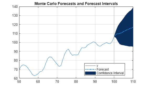
In this case, the MMSE and Monte Carlo forecasts and inferences are in close agreement.

More About MMSE and Monte Carlo Forecasting

Let y_t+ℓ denote the ℓ-step ahead forecast for the process (the prediction at time t + ℓ), conditioned on the history of the process up to time t (H_t) and exogenous covariate series up to time t + ℓ, x_{t + ℓ} when a regression component applies.

MMSE Forecasts

The ℓ-step-ahead minimum mean square error (MMSE) forecast is the value $${\widehat{y}}_{t+\ell }$$ that minimizes expected squared loss

$$E{\left(y_{t+\ell }-{\widehat{y}}_{t+\ell }|H_t,x_{t+\ell }\right)}^2.$$

The minimum of the expected squared loss is

$${\widehat{y}}_{t+\ell }=E(y_{t+\ell }|H_t,x_{t+\ell }).$$

The MMSE method provides an analytical solution to forecasting with appealing statistical properties. For more details, see [1], Ch. 5.1.

Forecast Mean Squared Error (MSE) and Inferences

The forecast mean square error for an ℓ-step ahead forecast is

$${\text{MSE}}_{\ell }=E{\left(y_{t+\ell }-{\widehat{y}}_{t+\ell }|H_{t+\ell -1},x_{t+\ell }\right)}^2.$$

To compute each MSE_ℓ, consider the infinite moving average (MA) process representation of the model y_t = c + x_t′β + ψ(L)ε_t, where $$\psi (L)=1+{\psi }_{1}L+{\psi }_2{L}^2+\dots$$. The sum of the variances of the lagged innovations yield the ℓ-step MSE

$$(1+{\psi }_1^2+{\psi }_2^2+\dots +{\psi }_{\ell -1}^2){\sigma }^2,$$

where σ² denotes the innovation variance.

The following results follow:

• For a stationary process, the coefficients of ψ(L) are absolutely summable and each MSE_ℓ converges to the unconditional variance of the process.

• For a nonstationary process, the sum of the coefficients of ψ(L) diverge; the forecast error grows without bound over time.

A 100(1 – ɑ)% confidence interval on the ℓ-step-ahead MMSE forecast is

$${\widehat{y}}_{T+\ell }\pm z_{\alpha /2}\sqrt{{\text{MSE}}_{\ell }},$$

where z_ɑ/2 is the z-score corresponding to the cumulative probability ɑ/2.

How forecast Generates MMSE Forecasts

The forecast function generates MMSE forecasts recursively because subsequent forecasts can require previous forecasts. For example, consider forecasting this AR(2) process from the end of the observed series at time T

$$y_t=c+{\varphi }_1{y}_{t-1}+{\varphi }_2{y}_{t-2}+{\epsilon }_t.$$

This model requires at least the p = 2 presample responses y_T–1 and y_Tforecast recursively generates forecasts as follows:

1. $${\widehat{y}}_{T+1}=c+{\varphi }_1{y}_T+{\varphi }_2{y}_{T-1}$$

2. $${\widehat{y}}_{T+2}=c+{\varphi }_1{\widehat{y}}_{T+1}+{\varphi }_2{y}_T$$

3. $${\widehat{y}}_{T+3}=c+{\varphi }_1{\widehat{y}}_{T+2}+{\varphi }_2{\widehat{y}}_{T+1}$$

4. In general, for the ℓ-step-ahead forecast, $${\widehat{y}}_{T+\ell }=c+{\varphi }_1{\widehat{y}}_{T+\ell -1}+{\varphi }_2{\widehat{y}}_{T+\ell -2}$$

For a stationary AR process, this recursion converges to the unconditional mean of the process,

$$\mu =\frac{c}{\left(1-{\varphi }_1-{\varphi }_2\right)}.$$

Similarly, for the MA(2) process

$$y_t=\mu +{\epsilon }_t+{\theta }_1{\epsilon }_{t-1}+{\theta }_2{\epsilon }_{t-2},$$

forecast requires q = 2 presample innovations to initialize the forecasts. By default, forecast sets all presample innovations from time T + 1 and greater to zero (their expected value). Thus, for an MA(2) process, the forecast for any time more than 2 steps in the future is the unconditional mean μ.

The equations imply that forecast requires a model Mdl, forecast horizon numperiods, and presample data, which are required to initialize the model for forecasting and indicate when the forecast period should begin.

The following conditions apply to presample data:

• The required number and type of presample observations depend on the model type and structure. In some cases, forecast sets default presample observations. Regardless, when you provide too few presample observations, forecast issues an error, and when you provide too many presample observations, forecast uses only the required number from the end of the series (for example, when two presample responses are required, forecast uses Y0((end-1):end) as a presample).

• For conditional mean models, Mdl.P specifies the minimum number of presample responses Y0.

• If the conditional mean model contains an MA component, forecast requires a minimum of Mdl.Q presample innovations E0. By default:

  • If you specify at least Mdl.P + Mdl.Q presample responses, forecast infers presample innovations (in this case, models containing an exogenous regression component require enough presample covariate data X0). In general, longer specified presample response series yield higher quality inferred presample innovations.

  • Otherwise, forecast sets all required presample innovations to 0.

• If the model variance is a conditional variance model, you must additionally account for any presample innovations or conditional variances V0 the conditional variance model requires.

If you forecast a model containing an exogenous regression component, forecast requires future exogenous covariate data XF for all steps in the forecast horizon. If you provide too few future exogenous covariate observations, forecast returns an error.

Monte Carlo Forecasts and Inferences

Monte Carlo forecasting uses Monte Carlo simulation to generate predictions; it is an alternative to MMSE forecasting. To generate the ℓ-step-ahead Monte Carlo forecast, for each ℓ in the forecast horizon, follow this general procedure:

1. Create a model. You can fully specify a model yourself, by calibrating all parameters, or fit a model to data by using the model's esimtate function (for example, see the estimate function for the arima model).

2. Obtain presample data to initialize the model for forecasting. For standard conditional mean models, the presample responses ate the last p observations in the response series. Conditional variance models can require presample innovations, which you can obtain by using the infer function.

3. Generate a large number of sample paths (for example, 1000) from the end of the series over the forecast horizon(as directed by the presample data). Each t = ℓ slice of the simulated paths in the forecast horizon composes an size 1000 sample from the distribution of the ℓ-step-ahead Monte Carlo forecast.

4. An ℓ-step-ahead Monte Carlo forecast is the mean of the associated sample. A 100(1 – ɑ)% confidence interval on the ℓ-step-ahead Monte Carlo forecast is the interval with the ɑ/2 and 1 – ɑ/2 quantiles as boundaries.

An advantage of Monte Carlo forecasting over MMSE forecasting is that you obtain a complete distribution for future events, not just a point estimate and standard error as provided by the MMSE method. By querying the entire distribution, you to answer more complex questions about the future than by using only point estimates and a standard error. Also, MMSE-based confidence intervals can contain unrealistic values, for example, the confidence interval can include negative values in an application where the response must be positive.

References

[1] Box, George E. P., Gwilym M. Jenkins, and Gregory C. Reinsel. Time Series Analysis: Forecasting and Control. 3rd ed. Englewood Cliffs, NJ: Prentice Hall, 1994.