Optimize Portfolio Using Fama-French Model

This example shows how to compare two approaches to optimize a portfolio with multiple risk factors. Both approaches use the Fama-French three-factor model to estimate risk in terms of size, value, and the overall return of the market.

• The first approach solves a tracking error problem based on prespecified factor exposure values and allows for improved performance metrics such as lower volatility.

• The second approach sets exact limits for factor exposure values, which guarantees target risk exposure, but can result in poor diversification.

For more information about this financial model, see Fama-French Three-Factor Model. For a mean-variance approach to portfolio optimization based on factors, see Portfolio Optimization Using Factor Models.

Solve Tracking Error Problem

Using this approach, you find a portfolio with a similar factor exposure to the target by solving a minimum tracking error problem.

Create a Portfolio object that includes stocks and Fama-French risk factors.

First, load one year of asset price data from the 30 component stocks of the Dow Jones Industrial Average (DJIA) market index. Separate the stock prices from the table and convert the prices to returns.

stockAndIndexPrices = readtimetable("dowPortfolio.xlsx");
stockPrices = stockAndIndexPrices(:,2:end);
stockReturns = tick2ret(stockPrices);
numStocks = width(stockReturns);

Load the three risk factors defined by the Fama-French model [1]:

• Excess Market Return (Mkt) — Represents the overall return of the market minus the one-month Treasury bill rate.

• Small Minus Big (SMB) — Reflects the excess returns of small-cap stocks over large-cap stocks.

• High Minus Low (HML) — Measures the difference in returns between high book-to-market (value) and low book-to-market (growth) stocks.

load("FamaFrench.mat")
numFactors = width(FamaFrenchThreeFactors);

Initialize a Portfolio object with both stock and factor returns.

returnsTT = synchronize(stockReturns,FamaFrenchThreeFactors, ...
    'intersection');
p = Portfolio;
p = estimateAssetMoments(p,returnsTT);

Set Portfolio Constraints

The factor returns are stored in the Portfolio object but are not investable assets. Use setBounds to set the lower and upper bounds to zero for the weights that correspond to the Fama-French factors. Set conditional bounds for any selected stock to be within 0.05 and 0.2.

lb = [0.05*ones(numStocks,1);zeros(numFactors,1)];
ub = [0.2*ones(numStocks,1);zeros(numFactors,1)];
boundType = [repmat("conditional",numStocks,1); ...
    repmat("simple",numFactors,1)];
p = setBounds(p,lb,ub,"BoundType",boundType);

Additionally, use setMinMaxNumAssets to limit the portfolio to hold a maximum of 10 assets. To ensure the solution is fully invested, sum all weights to 1 using setBudget.

p = setMinMaxNumAssets(p,0,10);
p = setBudget(p,1,1);

Calculate Optimal Portfolio

Define a target factor exposure for all three factors, then find the optimal asset allocation that minimizes the tracking error.

Represent the benchmark portfolio with zero weights on the stocks and the target exposure value for each of the three factors. The chosen values should result in a portfolio that positively correlates with the overall market, behaves more like large-cap stocks, and is slightly leaning toward value stocks instead of growth stocks.

marketExposure = 0.013;
SMBExposure = -0.003;
HMLExposure = 0.001;
targetFactorsExposure = [marketExposure;SMBExposure;HMLExposure];
wBmk = [zeros(numStocks,1);targetFactorsExposure];

Find the optimal investment strategy by solving a minimum tracking error problem. First, create the objective function.

TEObjective = @(w) 1e3*(w-wBmk)'*p.AssetCovar*(w-wBmk);

Set solver options for the Portfolio object using setSolverMINLP. Enable ExtendedFormulation. There are no nonlinear constraints, so set NumInnerCuts to zero. Then, solve the optimization problem using estimateCustomObjectivePortfolio and the custom tracking error function defined earlier, TEObjective.

p = setSolverMINLP(p,"OuterApproximation","ExtendedFormulation",true,...
    "NumInnerCuts",0);
wMinTE = estimateCustomObjectivePortfolio(p,TEObjective);

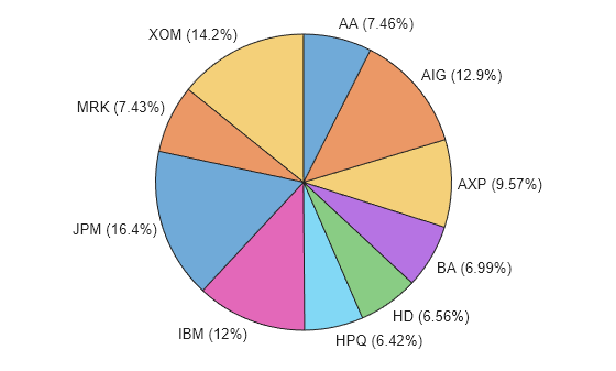
Plot the asset weights in a pie chart to visualize the portfolio.

idxMinTE = wMinTE >= 1e-4;
piechart(wMinTE(idxMinTE),returnsTT.Properties.VariableNames(idxMinTE))

Calculate Portfolio Factor Exposure

Use the factor loading matrix to calculate the factor exposure of the resulting portfolio.

To find the coefficients of the model, fit a linear model to each of the stocks.

Beta = zeros(numStocks,numFactors);
factorReturns = returnsTT{:,numStocks+1:end};
for i = 1:numStocks
    Beta(i,:) = factorReturns\stockReturns{:,i};
end

Plot the factor exposure for each stock selected by the optimal portfolio.

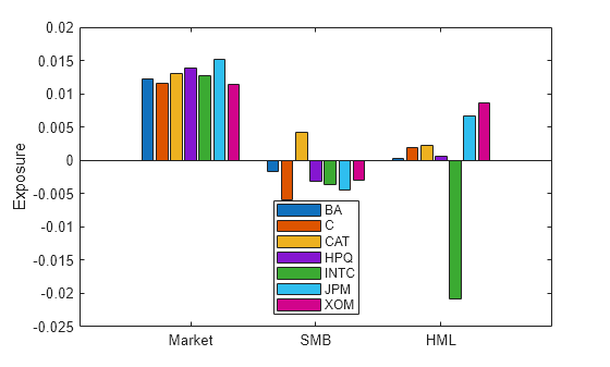
figure
bar(["Market","SMB","HML"],Beta(idxMinTE,:)')
legend(returnsTT.Properties.VariableNames(idxMinTE),"Location","north")
ylabel("Exposure")

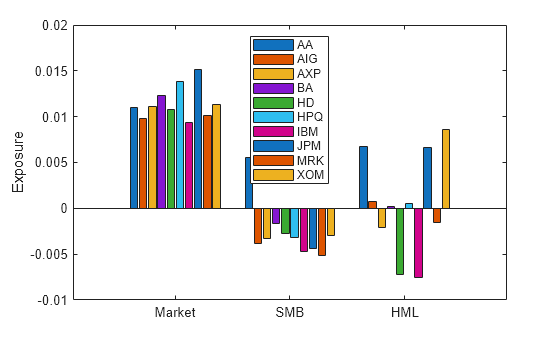
The plot shows that the portfolio selects stocks that have a market exposure between 0.0093 and 0.0151. Also, the portfolio selects stocks with both positive and negative exposure to the small-minus-big (SMB) and high-minus-low (HML) factors.

Now compute the overall portfolio exposure to each factor.

minTEExposure = Beta'*wMinTE(1:numStocks)

minTEExposure = 3×1

    0.0116
   -0.0030
    0.0013

The resulting portfolio exposures are close but do not exactly match the target exposures.

targetFactorsExposure

targetFactorsExposure = 3×1

    0.0130
   -0.0030
    0.0010

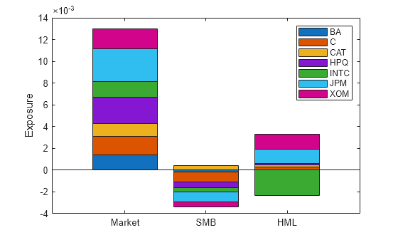
Plot the overall portfolio exposure as a stacked bar graph to show how each stock factor exposure contributes to the overall portfolio.

figure
weightedFactorExposure = Beta.*wMinTE(1:numStocks);
bar(["Market","SMB","HML"],weightedFactorExposure(idxMinTE,:)', ...
    'stacked')
legend(returnsTT.Properties.VariableNames(idxMinTE))
ylabel("Exposure")

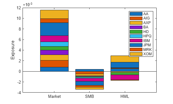
• For the excess market return (Market), the main contributors are JPM and XOM. Since the desired target exposure to the market is above average, the portfolio allocates a large share to JPM and XOM that have a higher-than-average market exposure.

• For SMB, there is only one stock in the portfolio with a positive exposure. This balances the rest of the negative contributions to achieve the SMB target exposure.

• For HML, the main contributors are also JPM and XOM, which have a large positive exposure to HML. This large positive exposure makes the overall exposure to HML above target.

Solve Exact Exposure Problem

The first approach shows how to find a portfolio with a similar factor exposure to the target by solving a minimum tracking error problem. In contrast, this approach calculates a portfolio with an exact factor exposure match to the target.

Create a new Portfolio object with the same constraints. The Portfolio object should consist only of stock returns.

q = Portfolio;
q = estimateAssetMoments(q,stockReturns);

q = setBounds(q,0.05,0.2,"BoundType","conditional");
q = setMinMaxNumAssets(q,0,10);
q = setBudget(q,1,1);

Use setEquality to set an equality constraint using the factor exposures. The constraint requires that the weighted sum of the stock factor exposures matches the target exposures.

q = setEquality(q,Beta',targetFactorsExposure);

Use estimateFrontierLimits to find the minimum risk portfolio that matches the target factor exposures exactly.

q = setSolverMINLP(q,"OuterApproximation","ExtendedFormulation",true, ...
    "NumInnerCuts",0,"ObjectiveScalingFactor",1e5);
wMinRisk = estimateFrontierLimits(q,'min');

Using this approach, the resulting portfolio factor exposures exactly match the target values because the problem uses an equality constraint.

minRiskExposure = Beta'*wMinRisk

minRiskExposure = 3×1

    0.0130
   -0.0030
    0.0010

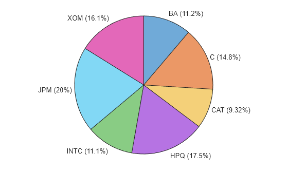
Plot the asset weights in a pie chart to visualize the portfolio.

idxMinRisk = wMinRisk >= 1e-4;
piechart(wMinRisk(idxMinRisk),returnsTT.Properties.VariableNames(idxMinRisk))

Plot the factor exposure for each stock.

figure
bar(["Market","SMB","HML"],Beta(idxMinRisk,:)')
legend(returnsTT.Properties.VariableNames(idxMinRisk),"Location","south")
ylabel("Exposure")

The plot shows that the portfolio selects stocks that have a market exposure between 0.0114 and 0.0151, which is a higher minimum than the tracking error market exposure. As in the previous section, the portfolio selects only one stock with a positive exposure to the small-minus-big (SMB) factor. In contrast, the portfolio only selects one stock with a negative high-minus-low (HML) factor.

Plot the overall portfolio exposure as a stacked bar graph to show how each stock factor exposure contributes to the overall portfolio.

figure
weightedFactorExposure = Beta.*wMinRisk(1:numStocks);
bar(["Market","SMB","HML"],weightedFactorExposure(idxMinRisk,:)', ...
    'stacked')
legend(returnsTT.Properties.VariableNames(idxMinRisk))
ylabel("Exposure")

• For the excess market return (Market), the stock contributions sum exactly to the target 0.013. The largest contributor is JPM as it has the highest market exposure.

• Only one stock has a positive exposure to the SMB factor with a small contribution compared to the remainder of the stocks. This is necessary to reach the target of -0.003.

• Only one stock has a negative exposure to HML. This negative exposure balances the rest of the positive exposures to reach a 0.001 exposure to the HML factor.

Compare Tracking Error and Exact Exposure Approaches

Compare the asset weight allocation of the two approaches by creating a bar graph.

figure
idxMinRisk = wMinRisk >= 1e-4;
idx = idxMinTE(1:numStocks) | idxMinRisk;
bar(returnsTT.Properties.VariableNames(idx),[wMinTE(idx) wMinRisk(idx)])
legend({"Tracking error","Exact exposure"},"Location","northwest")
ylabel("Weight")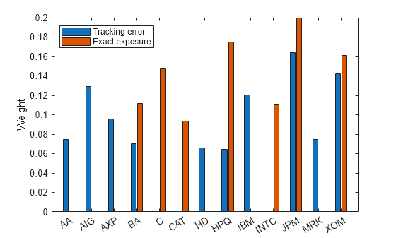

Each approach selects a different set and number of assets. For assets that are invested in both portfolios, the weight distribution is different.

The tracking error approach can deviate from the exact target values. This flexibility enables you to trade off between tracking error and factor exposures and potentially find a more efficient portfolio.

In contrast, the exact constraint approach guarantees that portfolio factor exposures are within the specified limits. For highly restrictive limits, portfolio optimization might result in suboptimal risk-return trade-offs, poor diversification, or infeasibility.

Note that different parameters, datasets, and solver options may lead to different computation times.

More About

Fama-French Three-Factor Model

The Fama-French three-factor model uses asset returns as a function of exposures to multiple systematic risk factors (market, size, value) [2]. This model enables you to see how much of your portfolio risk comes from each factor and to manage these exposures directly. Its formula is as follows:

$$r={\beta }_{\text{Mkt}}\left(\text{Mkt}\right)+{\beta }_{\text{SMB}}\left(\text{SMB}\right)+{\beta }_{\text{HML}}\left(\text{HML}\right)+\epsilon$$

where:

• $r$ is the rate of return.

• $\beta$ is the coefficient of the factor, or sensitivity.

• $\text{Mkt}$ is the excess market factor return.

• $\text{SMB}$ is the historic excess returns of small-cap companies over large cap companies.

• $\text{HML}$ is the historic excess returns of value stocks (high book-to-price ratio) over growth stocks (low book-to-price ratio).

• $\epsilon$ is the unexplained risk.

Factor Loading Matrix

The factor loading matrix represents the $\beta$ coefficients of the Fama-French three-factor model for each stock $i$ in the portfolio:

$$r_i={\beta }_{\left(i,\text{Mkt}\right)}\left(\text{Mkt}\right)+{\beta }_{\left(i,\text{SMB}\right)}\left(\text{SMB}\right)+{\beta }_{\left(i,\text{HML}\right)}\left(\text{HML}\right)+{\epsilon }_i$$

References

[1] Copyright Eugene F. Fama and Kenneth R. French. Used with permission; not for redistribution.

[2] Fama, Eugene F., and Kenneth R. French. “The Cross-Section of Expected Stock Returns.” The Journal of Finance, vol. 47, no. 2, June 1992, p. 427— 465.