gamultiobj

R2026b

Find Pareto front of multiple fitness functions using genetic algorithm

Syntax

x = gamultiobj(fun,nvars)

x = gamultiobj(fun,nvars,A,b)

x = gamultiobj(fun,nvars,A,b,Aeq,beq)

x = gamultiobj(fun,nvars,A,b,Aeq,beq,lb,ub)

x = gamultiobj(fun,nvars,A,b,Aeq,beq,lb,ub,nonlcon)

x = gamultiobj(fun,nvars,A,b,Aeq,beq,lb,ub,options)

x = gamultiobj(fun,nvars,A,b,Aeq,beq,lb,ub,nonlcon,options)

x = gamultiobj(fun,nvars,A,b,Aeq,beq,lb,ub,nonlcon,intcon)

x = gamultiobj(fun,nvars,A,b,Aeq,beq,lb,ub,nonlcon,intcon,options)

x = gamultiobj(problem)

[x,fval] = gamultiobj(___)

[x,fval,exitflag,output] = gamultiobj(___)

[x,fval,exitflag,output,population,scores] = gamultiobj(___)

Description

x = gamultiobj(fun,nvars) finds x on the Pareto Front of the objective functions defined in fun. nvars is the dimension of the optimization problem (number of decision variables). The solution x is local, which means it might not be on the global Pareto front.

Note

Passing Extra Parameters explains how to pass extra parameters to the objective function and nonlinear constraint functions, if necessary.

x = gamultiobj(fun,nvars,A,b) finds a local Pareto set x subject to the linear inequalities $$A\ast x\le b$$. See Linear Inequality Constraints. gamultiobj supports linear constraints only for the default PopulationType option ("doubleVector").

x = gamultiobj(fun,nvars,A,b,Aeq,beq) finds a local Pareto set x subject to the linear equalities $$Aeq\ast x=beq$$ and the linear inequalities $$A\ast x\le b$$, see Linear Equality Constraints. (Set A = [] and b = [] if no inequalities exist.) gamultiobj supports linear constraints only for the default PopulationType option ("doubleVector").

x = gamultiobj(fun,nvars,A,b,Aeq,beq,lb,ub) defines a set of lower and upper bounds on the design variables x so that a local Pareto set is found in the range lb ≤ x ≤ ub, see Bound Constraints. Use empty matrices for Aeq and beq if no linear equality constraints exist. gamultiobj supports bound constraints only for the default PopulationType option ("doubleVector").

x = gamultiobj(fun,nvars,A,b,Aeq,beq,lb,ub,nonlcon) finds a Pareto set subject to the constraints defined in nonlcon. The function nonlcon accepts x and returns vectors ineqnonlin and eqnonlin, representing the nonlinear inequalities and equalities respectively. gamultiobj minimizes fun such that ineqnonlin(x) ≤ 0 and eqnonlin(x) = 0. (Set lb = [] and ub = [] if no bounds exist.) gamultiobj supports nonlinear constraints only for the default PopulationType option ("doubleVector").

x = gamultiobj(fun,nvars,A,b,Aeq,beq,lb,ub,options) or x = gamultiobj(fun,nvars,A,b,Aeq,beq,lb,ub,nonlcon,options) finds a Pareto set x with the default optimization parameters replaced by values in options. Create options using optimoptions (recommended) or a structure.

x = gamultiobj(fun,nvars,A,b,Aeq,beq,lb,ub,nonlcon,intcon) or x = gamultiobj(fun,nvars,A,b,Aeq,beq,lb,ub,nonlcon,intcon,options) requires that the variables listed in intcon take integer values.

Note

When there are integer constraints, gamultiobj does not accept nonlinear equality constraints, only nonlinear inequality constraints.

x = gamultiobj(problem) finds the Pareto set for problem, where problem is a structure described in problem.

[x,fval] = gamultiobj(___), for any input variables, returns a matrix fval, the value of all the fitness functions defined in fun for all the solutions in x. fval has nf columns, where nf is the number of objectives, and has the same number of rows as x.

[x,fval,exitflag,output] = gamultiobj(___) returns exitflag, an integer identifying the reason the algorithm stopped, and output, a structure that contains information about the optimization process.

[x,fval,exitflag,output,population,scores] = gamultiobj(___) returns population, whose rows are the final population, and scores, the scores of the final population.

Examples

Simple Multiobjective Problem

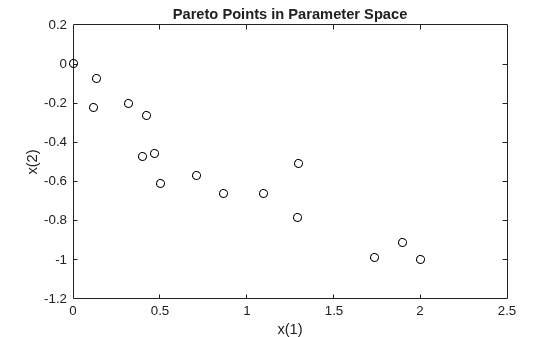
Find the Pareto front for a simple multiobjective problem. There are two objectives and two decision variables x.

fitnessfcn = @(x)[norm(x)^2,0.5*norm(x(:)-[2;-1])^2+2];

Find the Pareto front for this objective function.

rng default % For reproducibility
x = gamultiobj(fitnessfcn,2);

gamultiobj stopped because the average change in the spread of Pareto solutions is less than options.FunctionTolerance.

Plot the solution points.

plot(x(:,1),x(:,2),"ko")
xlabel("x(1)")
ylabel("x(2)")
title("Pareto Points in Parameter Space")

To see the effect of a linear constraint on this problem, see Multiobjective Problem with Linear Constraint.

Multiobjective Problem with Linear Constraint

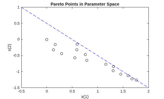
This example shows how to find the Pareto front for a multiobjective problem in the presence of a linear constraint.

There are two objective functions and two decision variables x.

fitnessfcn = @(x)[norm(x)^2,0.5*norm(x(:)-[2;-1])^2+2];

The linear constraint is $$x(1)+x(2)\le 1/2$$.

A = [1,1];
b = 1/2;

Find the Pareto front.

rng default % For reproducibility
x = gamultiobj(fitnessfcn,2,A,b);

gamultiobj stopped because the average change in the spread of Pareto solutions is less than options.FunctionTolerance.

Plot the constrained solution and the linear constraint.

plot(x(:,1),x(:,2),"ko")
t = linspace(-1/2,2);
y = 1/2 - t;
hold on
plot(t,y,"b--")
xlabel("x(1)")
ylabel("x(2)")
title("Pareto Points in Parameter Space")
hold off

To see the effect of removing the linear constraint from this problem, see Simple Multiobjective Problem.

Multiobjective Optimization with Bound Constraints

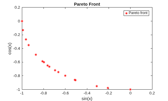
Find the Pareto front for the two fitness functions sin(x) and cos(x) on the interval $$0\le x\le 2\pi$$.

fitnessfcn = @(x)[sin(x),cos(x)];
nvars = 1;
lb = 0;
ub = 2*pi;
rng default % for reproducibility
x = gamultiobj(fitnessfcn,nvars,[],[],[],[],lb,ub)

gamultiobj stopped because the average change in the spread of Pareto solutions is less than options.FunctionTolerance.

x = 18×1

    4.7124
    4.7124
    3.1415
    3.6733
    3.9845
    3.4582
    3.9098
    4.4409
    4.0846
    3.8686
    4.1976
    4.0093
    4.5791
    3.6800
    4.0656
      ⋮

Plot the solution. gamultiobj finds points along the entire Pareto front.

plot(sin(x),cos(x),"r*")
xlabel("sin(x)")
ylabel("cos(x)")
title("Pareto Front")
legend("Pareto front")

Disconnected Pareto Front

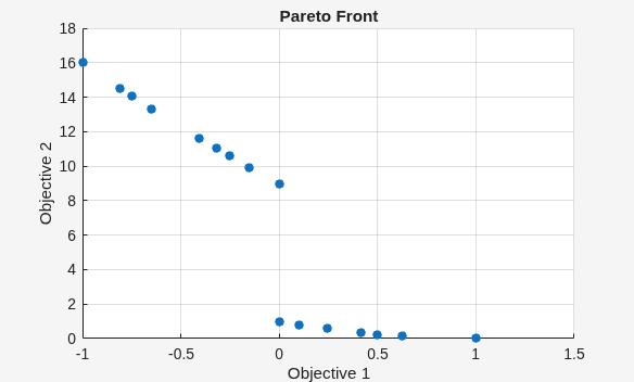
Find and plot the Pareto front for the two-objective Schaffer's second function. This function has a disconnected Pareto front.

Objective Function

The objective function schaffer2 has two columns of output representing two objectives.

function y = schaffer2(x) % y has two columns

% Initialize y for two objectives and for all x
y = zeros(length(x),2);

% Evaluate first objective.
% This objective is piecewise continuous.
for i = 1:length(x)
    if x(i) <= 1
        y(i,1) = -x(i);
    elseif x(i) <=3
        y(i,1) = x(i) -2;
    elseif x(i) <=4
        y(i,1) = 4 - x(i);
    else
        y(i,1) = x(i) - 4;
    end
end

% Evaluate second objective
y(:,2) = (x -5).^2;
end

Plot the Objectives

Plot the two objectives.

x = -1:0.1:8;
y = schaffer2(x);
plot(x,y(:,1),"r",x,y(:,2),"b");
xlabel("x")
ylabel("schaffer2(x)")
legend("Objective 1","Objective 2")

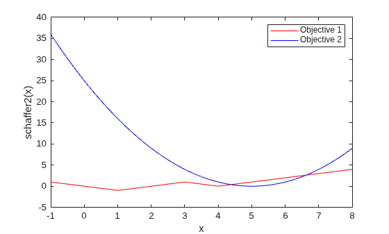
The two objective functions compete for x in the ranges [1,3] and [4,5]. But, the Pareto-optimal front consists of only two disconnected regions, corresponding to the x in the ranges [1,2] and [4,5]. There are disconnected regions because the region [2,3] is inferior to [4,5]. In that range, objective 1 has the same values, but objective 2 is smaller.

Run Multiobjective Optimization

Set bounds to keep population members in the range $$-5\le x\le 10$$.

lb = -5;
ub = 10;

Set options to view the Pareto front as gamultiobj runs.

options = optimoptions("gamultiobj",PlotFcn=@gaplotpareto);

Call gamultiobj.

rng default % For reproducibility
[x,fval,exitflag,output] = gamultiobj(@schaffer2,1,[],[],[],[],lb,ub,options);

gamultiobj stopped because it exceeded options.MaxGenerations.

Integer gamultiobj

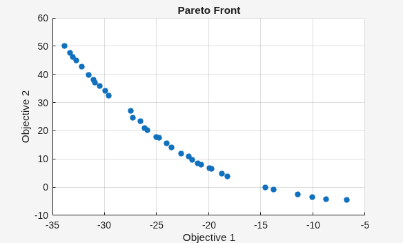
Create a two-objective function in two problem variables.

rng default % For reproducibility
M = diag([-1 -1]) + randn(2)/4; % Two problem variables
fun = @(x)[(x').^2 / 30 + M*x']; % Two objectives

Specify that the second variable must be an integer.

intcon = 2;

Specify problem bounds, the gaplotpareto plot function, and a population size of 100.

lb = [0 0];
ub = [100 50];
options = optimoptions("gamultiobj",PlotFcn="gaplotpareto",...
    PopulationSize=100);

Find the Pareto set for the problem.

nvars = 2;
A = [];
b = [];
Aeq = [];
beq = [];
nonlcon = [];
[x,fval] = gamultiobj(fun,nvars,A,b,Aeq,beq,lb,ub,nonlcon,intcon,options);

gamultiobj stopped because the average change in the spread of Pareto solutions is less than options.FunctionTolerance.

List ten of the solutions, and notice that the second variable is integer-valued.

x(1:10,:)

ans = 10×2

    8.3393   28.0000
   12.9927   49.0000
    7.1611   27.0000
    7.0210   18.0000
    0.0004   12.0000
    9.0989   44.0000
    9.3974   29.0000
    0.5537   17.0000
    6.4010   17.0000
    7.0531   31.0000

Obtain All Outputs from gamultiobj

Run a simple multiobjective problem and obtain all available outputs.

Set the random number generator for reproducibility.

rng default

Set the fitness functions to kur_multiobjective, a function listed at the end of this example that has three control variables and returns two fitness function values.

fitnessfcn = @kur_multiobjective;
nvars = 3;

Set lower and upper bounds on all variables.

ub = [5 5 5];
lb = -ub;

Find the Pareto front and all other outputs for this problem.

[x,fval,exitflag,output,population,scores] = gamultiobj(fitnessfcn,nvars, ...
    [],[],[],[],lb,ub);

gamultiobj stopped because the average change in the spread of Pareto solutions is less than options.FunctionTolerance.

Examine the sizes of some of the returned variables.

sizex = size(x)

sizex = 1×2

    18     3

sizepopulation = size(population)

sizepopulation = 1×2

    50     3

sizescores = size(scores)

sizescores = 1×2

    50     2

The returned Pareto front contains 18 points. There are 50 members of the final population. Each population row has three dimensions, corresponding to the three decision variables. Each scores row has two dimensions, corresponding to the two fitness functions.

function y = kur_multiobjective(x)
%KUR_MULTIOBJECTIVE Objective function for a multiobjective problem.
%   The Pareto-optimal set for this two-objective problem is nonconvex as
%   well as disconnected. The function KUR_MULTIOBJECTIVE computes two
%   objectives and returns a vector y of size 2-by-1.
%
%   Reference: Kalyanmoy Deb, "Multi-Objective Optimization using
%   Evolutionary Algorithms", John Wiley & Sons ISBN 047187339

%   Copyright 2007 The MathWorks, Inc.

% Initialize for two objectives
y = zeros(2,1);

% Compute first objective
for i = 1:2
    y(1) = y(1)  - 10*exp(-0.2*sqrt(x(i)^2 + x(i+1)^2));
end

% Compute second objective
for i = 1:3
    y(2) = y(2) +  abs(x(i))^0.8 + 5*sin(x(i)^3);
end
end

Input Arguments

fun — Fitness functions to optimize

function handle | function name

Fitness functions to optimize, specified as a function handle or function name.

fun is a function that accepts a real row vector of doubles x of length nvars and returns a real vector F(x) of objective function values. For details on writing fun, see Compute Objective Functions.

If you set the UseVectorized option to true, then fun accepts a matrix of size n-by-nvars, where the matrix represents n individuals. fun returns a matrix of size n-by-m, where m is the number of objective functions. See Vectorize the Fitness Function.

Example: @(x)[sin(x),cos(x)]

Data Types: char | function_handle | string

nvars — Number of variables

positive integer

Number of variables, specified as a positive integer. The solver passes row vectors of length nvars to fun.

Example: 4

Data Types: double

A — Linear inequality constraints

real matrix

Linear inequality constraints, specified as a real matrix. A is an M-by-nvars matrix, where M is the number of inequalities.

A encodes the M linear inequalities

A*x <= b,

where x is the column vector of nvars variables x(:), and b is a column vector with M elements.

For example, give constraints A = [1,2;3,4;5,6] and b = [10;20;30] to specify these sums:

x₁ + 2x₂ ≤ 10
3x₁ + 4x₂ ≤ 20
5x₁ + 6x₂ ≤ 30.

Example: To set the sum of the x-components to 1 or less, take A = ones(1,N) and b = 1.

Data Types: double

b — Linear inequality constraints

real vector

Linear inequality constraints, specified as a real vector. b is an M-element vector related to the A matrix. If you pass b as a row vector, solvers internally convert b to the column vector b(:).

b encodes the M linear inequalities

A*x <= b,

where x is the column vector of nvars variables x(:), and A is a matrix of size M-by-nvars.

For example, give constraints A = [1,2;3,4;5,6] and b = [10;20;30] to specify these sums:

x₁ + 2x₂ ≤ 10
3x₁ + 4x₂ ≤ 20
5x₁ + 6x₂ ≤ 30.

Example: To set the sum of the x-components to 1 or less, take A = ones(1,N) and b = 1.

Data Types: double

Aeq — Linear equality constraints

real matrix

Linear equality constraints, specified as a real matrix. Aeq is an Me-by-nvars matrix, where Me is the number of equalities.

Aeq encodes the Me linear equalities

Aeq*x = beq,

where x is the column vector of nvars variables x(:), and beq is a column vector with Me elements.

For example, give constraints Aeq = [1,2,3;2,4,1] and beq = [10;20] to specify these sums:

x₁ + 2x₂ + 3x₃ = 10
2x₁ + 4x₂ + x₃ = 20.

Example: To set the sum of the x-components to 1, take Aeq = ones(1,N) and beq = 1.

Data Types: double

beq — Linear equality constraints

real vector

Linear equality constraints, specified as a real vector. beq is an Me-element vector related to the Aeq matrix. If you pass beq as a row vector, solvers internally convert beq to the column vector beq(:).

beq encodes the Me linear equalities

Aeq*x = beq,

where x is the column vector of nvars variables x(:), and Aeq is a matrix of size Meq-by-N.

For example, give constraints Aeq = [1,2,3;2,4,1] and beq = [10;20] to specify these sums:

x₁ + 2x₂ + 3x₃ = 10
2x₁ + 4x₂ + x₃ = 20.

Example: To set the sum of the x-components to 1, take Aeq = ones(1,N) and beq = 1.

Data Types: double

lb — Lower bounds

real vector | real array

Lower bounds, specified as a real vector or real array. If numel(lb) = nvars, then lb specifies that x(i) >= lb(i) for all i.

If numel(lb) < nvars, then lb specifies that x(i) >= lb(i) for 1 <= i <= numel(lb).

In this case, solvers issue a warning.

Example: To specify all x-components as positive, set lb = zeros(nvars,1).

Data Types: double

ub — Upper bounds

real vector | real array

Upper bounds, specified as a real vector or real array. If numel(ub) = nvars, then ub specifies that x(i) <= ub(i) for all i.

If numel(ub) < nvars, then ub specifies that x(i) <= ub(i) for 1 <= i <= numel(ub).

In this case, solvers issue a warning.

Example: To specify all x-components as less than one, set ub = ones(nvars,1).

Data Types: double

nonlcon — Nonlinear constraints

function handle | function name

Nonlinear constraints, specified as a function handle or function name. nonlcon is a function that accepts a row vector x and returns two row vectors, ineqnonlin(x) and eqnonlin(x).

• ineqnonlin(x) is the vector of nonlinear inequality constraints at x. gamultiobj attempts to satisfy

  ineqnonlin(x) <= 0 for all entries of ineqnonlin.

• eqnonlin(x) is the vector of nonlinear equality constraints at x. gamultiobj attempts to satisfy

  eqnonlin(x) = 0 for all entries of eqnonlin.

For example,

  x = gamultiobj(@myfun,x0,...,@mycon)

where mycon is a MATLAB^® function such as the following:

function [ineqnonlin,eqnonlin] = mycon(x)
ineqnonlin = ...     % Compute nonlinear inequalities at x.
eqnonlin = ...   % Compute nonlinear equalities at x.

If you set the UseVectorized option to true, then nonlcon accepts a matrix of size n-by-nvars, where the matrix represents n individuals. nonlcon returns a matrix of size n-by-mc in the first argument, where mc is the number of nonlinear inequality constraints. nonlcon returns a matrix of size n-by-mceq in the second argument, where mceq is the number of nonlinear equality constraints. See Vectorize the Fitness Function.

For more information, see Nonlinear Constraints.

Data Types: char | function_handle | string

options — Optimization options

output of optimoptions | structure

Optimization options, specified as the output of optimoptions or a structure. See option details in Genetic Algorithm Options.

optimoptions hides the options listed in italics. See Options That optimoptions Hides.

Options for ga and gamultiobj

Option	Description		Values
ConstraintTolerance	Determines the feasibility with respect to nonlinear constraints. Also, max(sqrt(eps),ConstraintTolerance) determines feasibility with respect to linear constraints. Default: 1e-3. For an options structure, use TolCon.		Nonnegative scalar
CreationFcn	Function that creates the initial population. Specify as a name of a built-in creation function or a function handle. See Population Options. Defaults:		Choose any of these: "gacreationuniform" | "gacreationlinearfeasible" | "gacreationnonlinearfeasible" | "gacreationuniformint" | "gacreationsobol" | Custom creation function
	ga with constraints: Integer: "gacreationuniformint" Else nonlinear with NonlinearConstraintAlgorithm="penalty": "gacreationnonlinearfeasible" Else linear: "gacreationlinearfeasible" Otherwise: "gacreationuniform"	gamultiobj with constraints: Integer: "gacreationsobol" Else linear: "gacreationlinearfeasible" Otherwise: "gacreationuniform"
CrossoverFcn	Function that the algorithm uses to create crossover children. Specify as a name of a built-in crossover function or a function handle. See Crossover Options. Defaults:		Choose any of these: "crossoverscattered" | "crossoverintermediate" | "crossoverlaplace" | "crossoverheuristic" | "crossoversinglepoint" | "crossovertwopoint" | "crossoverarithmetic" | Custom crossover function
	ga with constraints: Integer: "crossoverlaplace" Else linear: "crossoverintermediate" Otherwise: "crossoverscattered"	gamultiobj with constraints: Integer or linear: "crossoverintermediate" Otherwise: "crossoverscattered"
CrossoverFraction	The fraction of the population at the next generation, not including elite children, that the crossover function creates. Default: 0.8.		Nonnegative scalar
Display	Level of display. Default: "final".		"off" | "iter" | "diagnose" | "final"
DistanceMeasureFcn	Function that computes the distance measure of individuals. Specify as a name of a built-in distance measure function or a function handle. The value applies to the decision variable or design space (genotype) or to function space (phenotype). The default "distancecrowding" is in function space (phenotype). For gamultiobj only. See Multiobjective Options. For an options structure, use a function handle, not a name.		"distancecrowding" means the same as @distancecrowding,"phenotype" | @distancecrowding,"genotype" | Custom distance function
EliteCount	Positive integer specifying how many individuals in the current generation are guaranteed to survive to the next generation. Not used in gamultiobj. Default: ceil(0.05*PopulationSize).		Nonnegative integer
FitnessLimit	If the fitness function attains the value of FitnessLimit, the algorithm halts. Not used in gamultiobj. Default: -Inf.		Scalar
FitnessScalingFcn	Function that scales the values of the fitness function. Specify as a name of a built-in scaling function or a function handle. Not used in gamultiobj.		"fitscalingrank" | "fitscalingshiftlinear" | "fitscalingprop" | "fitscalingtop" | Custom fitness scaling function
FunctionTolerance	The algorithm stops if the average relative change in the best fitness function value over MaxStallGenerations generations is less than or equal to FunctionTolerance. If StallTest is "geometricWeighted", then the algorithm stops if the weighted average relative change is less than or equal to FunctionTolerance. For gamultiobj, the algorithm stops when the geometric average of the relative change in value of the spread over options.MaxStallGenerations generations is less than options.FunctionTolerance, and the final spread is less than the mean spread over the past options.MaxStallGenerations generations. See gamultiobj Algorithm. For an options structure, use TolFun.		Nonnegative scalar | 1e-6 for ga, 1e-4 for gamultiobj
HybridFcn	Function that continues the optimization after ga terminates. Specify as a name or a function handle. Alternatively, a cell array specifying the hybrid function and its options. See ga Hybrid Function. For gamultiobj, the only hybrid function is @fgoalattain. See gamultiobj Hybrid Function. When the problem has integer constraints, you cannot use a hybrid function. See When to Use a Hybrid Function.		Function name or handle | "fminsearch" | "patternsearch" | "fminunc" | "fmincon" | [] or 1-by-2 cell array | @solver, hybridoptions, where solver = fminsearch, patternsearch, fminunc, or fmincon []
InitialPenalty	Initial value of the penalty parameter. Not used in gamultiobj. Default: 10.		Positive scalar
InitialPopulationMatrix	Initial population used to seed the genetic algorithm. Has up to PopulationSize rows and N columns, where N is the number of variables. You can pass a partial population, meaning one with fewer than PopulationSize rows. In that case, the genetic algorithm uses CreationFcn to generate the remaining population members. See Population Options. Default: []. For an options structure, use InitialPopulation.		Matrix
InitialPopulationRange	Matrix or vector specifying the range of the individuals in the initial population. Applies to gacreationuniform creation function. ga shifts and scales the default initial range to match any finite bounds. Default: [-10;10] for unbounded components, [-1e4+1;1e4+1] for unbounded components of integer-constrained problems, [lb;ub] for bounded components, with the default range modified to match one-sided bounds. For an options structure, use PopInitRange.		Matrix or vector
InitialScoresMatrix	Initial scores used to determine fitness. Has up to PopulationSize rows and Nf columns, where Nf is the number of fitness functions (1 for ga, greater than 1 for gamultiobj). You can pass a partial scores matrix, meaning one with fewer than PopulationSize rows. In that case, the solver fills in the scores when it evaluates the fitness functions. Default: []. For an options structure, use InitialScores.		Column vector for single objective | matrix for multiobjective
MaxGenerations	Maximum number of iterations before the algorithm halts. Default: 100*numberOfVariables for ga, 200*numberOfVariables for gamultiobj. For an options structure, use Generations.		Nonnegative integer
MaxStallGenerations	The algorithm stops if the average relative change in the best fitness function value over MaxStallGenerations generations is less than or equal to FunctionTolerance. If StallTest is "geometricWeighted", then the algorithm stops if the weighted average relative change is less than or equal to FunctionTolerance. For gamultiobj, the algorithm stops when the geometric average of the relative change in value of the spread over options.MaxStallGenerations generations is less than options.FunctionTolerance, and the final spread is less than the mean spread over the past options.MaxStallGenerations generations. See gamultiobj Algorithm. Default: 50 for ga, 100 for gamultiobj. For an options structure, use StallGenLimit.		Nonnegative integer
MaxStallTime	The algorithm stops if there is no improvement in the objective function for MaxStallTime, a duration measured by tic and toc. Not used in gamultiobj. If you specify a scalar value, the value becomes a duration with the unit seconds. Default: Inf. For an options structure, use a scalar StallTimeLimit.		duration | Positive scalar
MaxTime	Maximum amount of time that the algorithm runs as measured by tic and toc, a duration or Inf. The default is Inf, which disables this stopping criterion. The limit is enforced after each iteration, so the solver can exceed the limit. If you specify a scalar value, the value becomes a duration with the unit seconds. For an options structure, use a scalar TimeLimit.		duration | Nonnegative scalar
MigrationDirection	Direction of migration. Default: "forward". See Migration Options.		"both" | "forward"
MigrationFraction	Scalar from 0 through 1 specifying the fraction of individuals in each subpopulation that migrates to a different subpopulation. Default: 0.2. See Migration Options.		Scalar
MigrationInterval	Positive integer specifying the number of generations that take place between migrations of individuals between subpopulations. Default: 20. See Migration Options.		Positive integer
MutationFcn	Function that produces mutation children. Specify as a name of a built-in mutation function or a function handle. See Mutation Options. Defaults:		Choose any of these: "mutationgaussian" | "mutationadaptfeasible" | "mutationpower" | "mutationpositivebasis" | "mutationuniform" | Custom mutation function
	ga with constraints: Integer: "mutationpower" Else linear or bounds: "mutationadaptfeasible" Otherwise: "mutationgaussian"	gamultiobj with constraints: Integer: "mutationpositivebasis" Else linear or bounds: "mutationadaptfeasible" Otherwise: "mutationgaussian"
NonlinearConstraintAlgorithm	Nonlinear constraint algorithm. See Nonlinear Constraint Solver Algorithms for Genetic Algorithm. Option unchangeable for gamultiobj. Default: "auglag". For an options structure, use NonlinConAlgorithm.		"auglag" | "penalty"
OutputFcn	Functions that the solver calls at each iteration. Specify as a function handle or a cell array of function handles. Default: []. See Output Function Options. For an options structure, use OutputFcns.		Function handle or cell array of function handles
ParetoFraction	Scalar from 0 through 1 specifying the fraction of individuals to keep on the first Pareto front while the solver selects individuals from higher fronts, for gamultiobj only. Default: 0.35. See Multiobjective Options.		Scalar |
PenaltyFactor	Penalty update parameter. Not used in gamultiobj. Default: 100.		Positive scalar
PlotFcn	Function that plots data computed by the algorithm. Specify as a name of a built-in plot function, a function handle, or a cell array of built-in names or function handles. See Plot Options. For an options structure, use PlotFcns.		ga or gamultiobj: [] | "gaplotdistance" | "gaplotselection" | "gaplotscorediversity" |"gaplotscores" | "gaplotstopping" | "gaplotmaxconstr" | Custom plot function ga only: "gaplotbestf" | "gaplotbestindiv" | "gaplotexpectation" | "gaplotgenealogy" | "gaplotrange" gamultiobj only: "gaplotpareto" | "gaplotparetodistance" | "gaplotrankhist" | "gaplotspread"
PlotInterval	Positive integer specifying the number of generations between consecutive calls to the plot functions. Default: 1.		Positive integer
PopulationSize	Size of the population. Default: 50 when numberOfVariables <= 5, 200 otherwise. The default for ga only with a mixed-integer problem, min(max(10*nvars,40),100).		Positive integer
PopulationType	Data type of the population. Must be "doubleVector" for mixed-integer problems. Default: "doubleVector". ga ignores all constraints when PopulationType is set to "bitString" or "custom". See Population Options.		"bitstring" | "custom" | "doubleVector"
SelectionFcn	Function that selects parents of crossover and mutation children. Specify as a name of a built-in selection function or a function handle. Defaults:		For ga, choose any of these: "selectionstochunif" | "selectiontournament" | "selectionremainder" | "selectionuniform" | "selectionroulette" | Custom selection function
	ga with constraints: Integer or nonlinear penalty: "selectiontournament" Otherwise: "selectionstochunif"	gamultiobj uses only "selectiontournament" or a custom selection function
StallTest	Stopping test type. Not used in gamultiobj. Default: "averageChange".		"geometricWeighted" | "averageChange"
UseParallel	Compute fitness and nonlinear constraint functions in parallel. Option for using parallel computing, specified as one of these values: "auto" — If a parallel pool is open or automatic pool creation is enabled, compute in parallel. Otherwise, compute serially. "on" — Compute in parallel. If no parallel pool is open, the solver starts one using your default cluster profile. "off" — Compute serially. The default is "off". To use a parallel pool to run computations in MATLAB, you must have Parallel Computing Toolbox™. The values true and false are also accepted for backward compatibility. true maps to "auto" and false maps to "off". See Vectorize and Parallel Options (User Function Evaluation) and Parallel Computing in Global Optimization Toolbox.		"auto" | "on" | {"off"}
UseVectorized	Specifies whether functions are vectorized. Default: false. See Vectorize and Parallel Options (User Function Evaluation) and Vectorize the Fitness Function. For an options structure, use Vectorized with the values "on" or "off".		true | false

Example: optimoptions("gamultiobj",PlotFcn=@gaplotpareto)

intcon — Integer variables

vector of positive integers

Integer variables, specified as a vector of positive integers taking values from 1 to nvars. Each value in intcon represents an x component that is integer-valued.

Note

When intcon is nonempty, nonlcon must return empty for eqnonlin.

Example: To specify that the even entries in x are integer-valued, set intcon to 2:2:nvars

Data Types: double

problem — Problem description

structure

Problem description, specified as a structure containing these fields.

fitnessfcn	Fitness functions
nvars	Number of design variables
Aineq	A matrix for linear inequality constraints
Bineq	b vector for linear inequality constraints
Aeq	Aeq matrix for linear equality constraints
Beq	beq vector for linear equality constraints
lb	Lower bound on x
ub	Upper bound on x
nonlcon	Nonlinear constraint functions
intcon	Indices of integer variables
rngstate	Field to reset the state of the random number generator
solver	"gamultiobj"
options	Options created using optimoptions or an options structure

You must specify the fields fitnessfcn, nvars, and options. The remainder are optional for gamultiobj.

Data Types: struct

Output Arguments

x — Pareto points

m-by-nvars array

Pareto points, returned as an m-by-nvars array, where m is the number of points on the Pareto front. Each row of x represents one point on the Pareto front.

fval — Function values on Pareto front

m-by-nf array

Function values on the Pareto front, returned as an m-by-nf array. m is the number of points on the Pareto front, and nf is the number of fitness functions. Each row of fval represents the function values at one Pareto point in x.

exitflag — Reason gamultiobj stopped

integer

Reason gamultiobj stopped, returned as an integer.

exitflag Value	Stopping Condition
1	Geometric average of the relative change in value of the spread over options.MaxStallGenerations generations is less than options.FunctionTolerance, and the final spread is less than the mean spread over the past options.MaxStallGenerations generations
0	Maximum number of generations exceeded
-1	Optimization terminated by an output function or plot function
-2	No feasible point found
-5	Time limit exceeded

output — Information about the optimization process

structure

Information about the optimization process, returned as a structure with these fields.

output Field	Meaning
problemtype	Type of problem: "unconstrained" — No constraints "boundconstraints" — Only bound constraints "linearconstraints" — Linear constraints, with or without bound constraints "nonlinearconstr" — Nonlinear constraints, with or without other types of constraints
rngstate	State of the MATLAB random number generator, just before the algorithm started. You can use the values in rngstate to reproduce the output of gamultiobj. See Reproduce Results.
generations	Total number of generations, excluding HybridFcn iterations.
funccount	Total number of function evaluations.
message	gamultiobj exit message.
stddistance	Standard deviation of “distance,” which by default is the standard deviation of the norm of the difference between Pareto front members and their mean.
spread	Combination of the “distance,” and a measure of the movement of the points on the Pareto front between the final two iterations.
maxconstraint	Maximum constraint violation at the final Pareto set.

population — Final population

n-by-nvars array

Final population, returned as an n-by-nvars array, where n is the number of members of the population.

scores — Scores of the final population

n-by-nf array

Scores of the final population, returned as an n-by-nf array. n is the number of members of the population, and nf is the number of fitness functions.

When there are nonlinear constraints, gamultiobj sets the scores of infeasible population members to Inf.

More About

Pareto Front

A Pareto front is a set of points in parameter space (the space of decision variables) that have noninferior fitness function values.

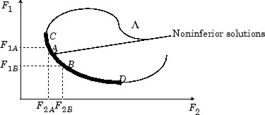
In other words, for each point on the Pareto front, you can improve one fitness function only by degrading another. For details, see What Is Multiobjective Optimization?

As in Local vs. Global Optima, it is possible for a Pareto front to be local, but not global. “Local” means that the Pareto points can be noninferior compared to nearby points, but points farther away in parameter space could have lower function values in every component.

Algorithms

gamultiobj uses a controlled, elitist genetic algorithm (a variant of NSGA-II [1]). An elitist GA always favors individuals with better fitness value (rank). A controlled elitist GA also favors individuals that can help increase the diversity of the population even if they have a lower fitness value. It is important to maintain the diversity of population for convergence to an optimal Pareto front. Diversity is maintained by controlling the elite members of the population as the algorithm progresses. Two options, ParetoFraction and DistanceMeasureFcn, control the elitism. ParetoFraction limits the number of individuals on the Pareto front (elite members). The distance function, selected by DistanceMeasureFcn, helps to maintain diversity on a front by favoring individuals that are relatively far away on the front. The algorithm stops if the spread, a measure of the movement of the Pareto front, is small. For details, see gamultiobj Algorithm.

Alternative Functionality

App

The Optimize Live Editor task provides a visual interface for gamultiobj.

References

[1] Deb, Kalyanmoy. Multi-Objective Optimization Using Evolutionary Algorithms. Chichester, England: John Wiley & Sons, 2001.

Extended Capabilities

Automatic Parallel Support

Accelerate code by automatically running computation in parallel using Parallel Computing Toolbox™.

To run in parallel, set the UseParallel option to "auto" or "on".

options = optimoptions("solvername",UseParallel="auto")

For more information, see Parallel Computing in Global Optimization Toolbox.

Version History

Introduced in R2007b

R2026b: Specify MaxTime option as duration

Specify the MaxTime option as a duration, or as a scalar that is interpreted as a duration in seconds. For example,

options.MaxTime = minutes(3);

Previously, MaxTime was a scalar, the number of seconds.

R2026a: Updates to custom creation, crossover, and mutation functions, and updates to options in custom selection and distance measure functions

Custom creation, crossover, and mutation functions in ga and gamultiobj now have a problem structure argument instead of FitnessFcn. To access the value of FitnessFcn, use problem.FitnessFcn. The passed problem structure has an empty options field because the options are passed in a separate argument. For syntax details, see Genetic Algorithm Options.

Additionally, all these custom functions plus custom selection functions and, for gamultiobj, custom distance measure functions, now include options passed as an optimoptions object. This change makes it easier to create and update options in custom functions by using the current documented names. You can also use legacy option names; see Current and Legacy Option Names.