Plot 3-D Pareto Front

R2026b

This example shows how to plot a Pareto front for three objectives. Each objective function is the squared distance from a particular 3-D point. For speed of calculation, write each objective function in vectorized fashion as a dot product. To obtain a dense solution set, use 200 points on the Pareto front.

The example first shows how to obtain the plot using the built-in "psplotparetof" plot function. Then solve the same problem and obtain the plot using gamultiobj, which requires slightly different option settings. The example shows how to obtain solution variables for a particular point in the Pareto plot. Then the example shows how to plot the points directly, without using a plot function, and shows how to plot an interpolated surface instead of Pareto points.

fun = @(x)[dot(x - [1,2,3],x - [1,2,3],2), ...
    dot(x - [-1,3,-2],x - [-1,3,-2],2), ...
    dot(x - [0,-1,1],x - [0,-1,1],2)];
options = optimoptions("paretosearch",UseVectorized=true,ParetoSetSize=200,...
    PlotFcn="psplotparetof");
lb = -5*ones(1,3);
ub = -lb;
rng default % For reproducibility
[x,f] = paretosearch(fun,3,[],[],[],[],lb,ub,[],options);

Pareto set found that satisfies the constraints. 

Optimization completed because the relative change in the volume of the Pareto set 
is less than 'options.ParetoSetChangeTolerance' and constraints are satisfied to within 
'options.ConstraintTolerance'.

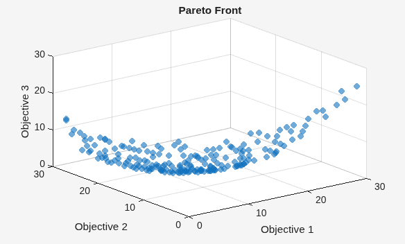
opts = optimoptions("gamultiobj",PlotFcn="gaplotpareto",PopulationSize=200);
[xg,fg] = gamultiobj(fun,3,[],[],[],[],lb,ub,[],opts);

gamultiobj stopped because the average change in the spread of Pareto solutions is less than options.FunctionTolerance.

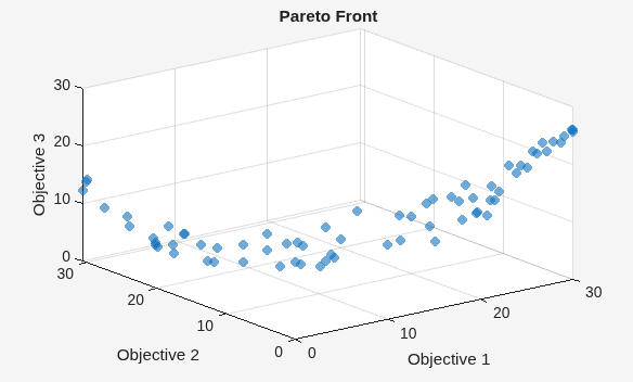
This plot shows many fewer points than the paretosearch plot. Solve the problem again using a larger population.

opts.PopulationSize = 400;
[xg,fg] = gamultiobj(fun,3,[],[],[],[],lb,ub,[],opts);

gamultiobj stopped because the average change in the spread of Pareto solutions is less than options.FunctionTolerance.

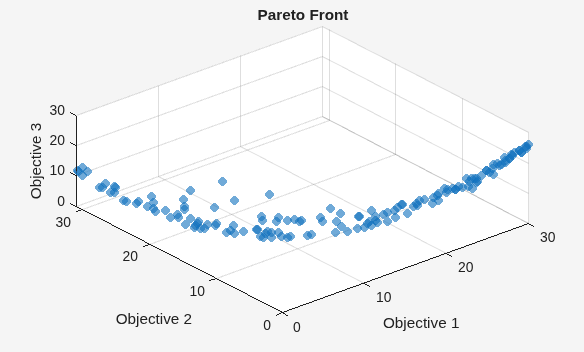
Change the viewing angle to better match the psplotpareto plot.

view(-40,57)

Find Solution Point Using Data Tips

Select a point in the plot by using the Data Tips tool.

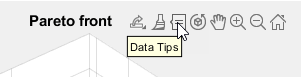
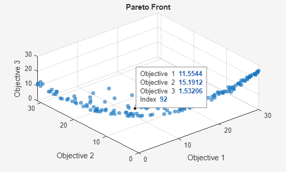
The pictured point has index 92. Display the point xg(92,:) that contains the solution variables associated with the pictured point.

disp(xg(92,:))

   -0.2889    0.0939    0.4980

Evaluate the objective functions at this point to see that it matches the displayed values.

disp(fun(xg(92,:)))

   11.5544   15.1912    1.5321

Create 3-D Scatter Plot

Plot points on the Pareto front by using scatter3.

figure
subplot(2,2,1)
scatter3(f(:,1),f(:,2),f(:,3),".");
subplot(2,2,2)
scatter3(f(:,1),f(:,2),f(:,3),".");
view(-148,8)
subplot(2,2,3)
scatter3(f(:,1),f(:,2),f(:,3),".");
view(-180,8)
subplot(2,2,4)
scatter3(f(:,1),f(:,2),f(:,3),".");
view(-300,8)

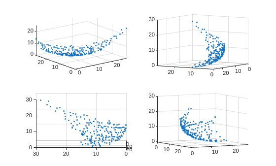
By rotating the plot interactively, you get a better view of its structure.

Interpolated Surface Plot

To see the Pareto front as a surface, create a scattered interpolant.

figure
F = scatteredInterpolant(f(:,1),f(:,2),f(:,3),"linear","none");

To plot the resulting surface, create a mesh in x-y space from the smallest to the largest values. Then plot the interpolated surface.

sgr = linspace(min(f(:,1)),max(f(:,1)));
ygr = linspace(min(f(:,2)),max(f(:,2)));
[XX,YY] = meshgrid(sgr,ygr);
ZZ = F(XX,YY);

Plot the Pareto points and surface together.

figure
subplot(2,2,1)
surf(XX,YY,ZZ,LineStyle="none")
hold on
scatter3(f(:,1),f(:,2),f(:,3),".");
hold off
subplot(2,2,2)
surf(XX,YY,ZZ,LineStyle="none")
hold on
scatter3(f(:,1),f(:,2),f(:,3),".");
hold off
view(-148,8)
subplot(2,2,3)
surf(XX,YY,ZZ,LineStyle="none")
hold on
scatter3(f(:,1),f(:,2),f(:,3),".");
hold off
view(-180,8)
subplot(2,2,4)
surf(XX,YY,ZZ,LineStyle="none")
hold on
scatter3(f(:,1),f(:,2),f(:,3),".");
hold off
view(-300,8)

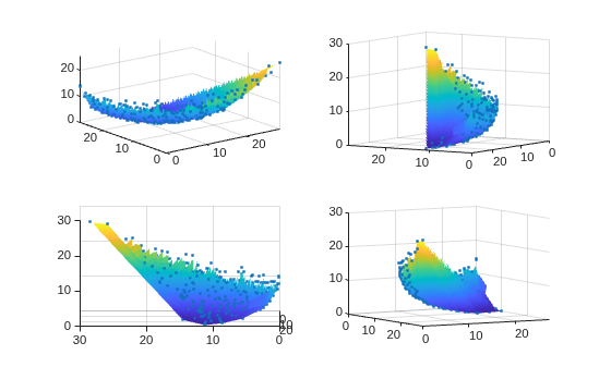
By rotating the plot interactively, you get a better view of its structure.

Plot Pareto Set in Control Variable Space

You can obtain a plot of the points on the Pareto set by using the "psplotparetox" plot function.

options.PlotFcn = "psplotparetox";
[x,f] = paretosearch(fun,3,[],[],[],[],lb,ub,[],options);

Pareto set found that satisfies the constraints. 

Optimization completed because the relative change in the volume of the Pareto set 
is less than 'options.ParetoSetChangeTolerance' and constraints are satisfied to within 
'options.ConstraintTolerance'.

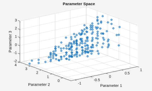
Alternatively, create a scatter plot of the x-values in the Pareto set.

figure
subplot(2,2,1)
scatter3(x(:,1),x(:,2),x(:,3),".");
subplot(2,2,2)
scatter3(x(:,1),x(:,2),x(:,3),".");
view(-148,8)
subplot(2,2,3)
scatter3(x(:,1),x(:,2),x(:,3),".");
view(-180,8)
subplot(2,2,4)
scatter3(x(:,1),x(:,2),x(:,3),".");
view(-300,8)

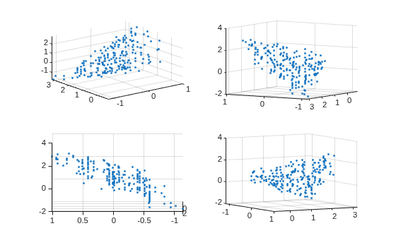
This set does not have a clear surface. By rotating the plot interactively, you get a better view of its structure.

Parallel Plot

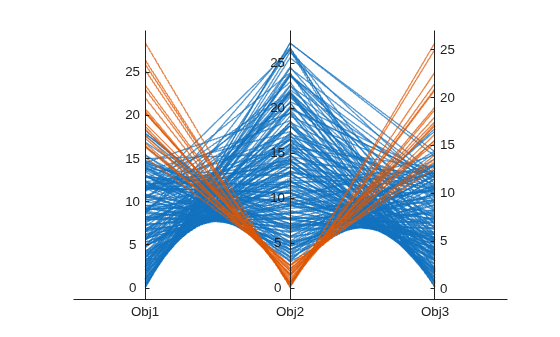
You can plot the Pareto set using a parallel coordinates plot. You can use a parallel coordinates plot for any number of dimensions. In the plot, each colored line represents one Pareto point, and each coordinate variable plots to an associated vertical line. Plot the objective function values using parellelplot.

figure
p = parallelplot(f);
p.CoordinateTickLabels = ["Obj1";"Obj2";"Obj3"];

Color the Pareto points in the lowest tenth of the values of Obj2.

minObj2 = min(f(:,2));
maxObj2 = max(f(:,2));
grpRng = minObj2 + 0.1*(maxObj2-minObj2);
grpData = f(:,2) <= grpRng;
p.GroupData = grpData;
p.LegendVisible = "off";