Gradual Area Change

(To be removed) Gradual enlargement or contraction

The Hydraulics (Isothermal) library will be removed in a future release. Use the Isothermal Liquid library instead. (since R2020a)

For more information on updating your models, see Upgrading Hydraulic Models to Use Isothermal Liquid Blocks.

• 

Libraries:
Simscape / Fluids / Hydraulics (Isothermal) / Local Hydraulic Resistances

Description

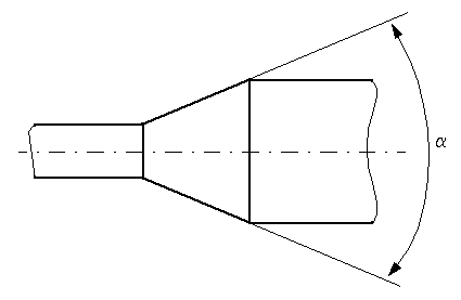
The Gradual Area Change block represents a local hydraulic resistance, such as a gradual cross-sectional area change. The resistance represents a gradual enlargement (diffuser) if fluid flows from inlet to outlet, or a gradual contraction if fluid flows from outlet to inlet. The block is based on the Local Resistance block. It determines the pressure loss coefficient and passes its value to the underlying Local Resistance block. The block offers two methods of parameterization: by applying semi-empirical formulas (with a constant value of the pressure loss coefficient) or by table lookup for the pressure loss coefficient based on the Reynolds number.

If you choose to apply the semi-empirical formulas, you provide geometric parameters of the resistance, and the pressure loss coefficient is determined according to the A.H. Gibson equations (see [1] and [2]):

$$K_{GE}=\{\begin{array}{ll}{K}_{cor}{\left(1-\frac{A_s}{A_L}\right)}^2·2.6\sin \frac{\alpha }{2}\hfill & \text{for 0 < }\alpha \text{ <= }{45}^o\hfill \\ K_{cor}{\left(1-\frac{A_s}{A_L}\right)}^2\hfill & \text{for }{45}^o\text{ < }\alpha \text{ < }{180}^o\hfill \end{array}$$

$$K_{GC}=\{\begin{array}{ll}{K}_{cor}·0.5{\left(1-\frac{A_s}{A_L}\right)}^{0.75}·1.6\sin \frac{\alpha }{2}\hfill & \text{for 0 < }\alpha \text{ <= }{45}^o\hfill \\ K_{cor}·0.5{\left(1-\frac{A_s}{A_L}\right)}^{0.75}·\sqrt{\sin \frac{\alpha }{2}}\hfill & \text{for }{45}^o\text{ < }\alpha \text{ < }{180}^o\hfill \end{array}$$

where

KGE	Pressure loss coefficient for the gradual enlargement, which takes place if fluid flows from inlet to outlet
KGC	Pressure loss coefficient for the gradual contraction, which takes place if fluid flows from outlet to inlet
Kcor	Correction factor
AS	Small area
AL	Large area
α	Enclosed angle

If you choose to specify the pressure loss coefficient by a table, you have to provide a tabulated relationship between the loss coefficient and the Reynolds number. In this case, the loss coefficient is determined by one-dimensional table lookup. You have a choice of two interpolation methods and two extrapolation methods.

The pressure loss coefficient, determined by either of the two methods, is then passed to the underlying Local Resistance block, which computes the pressure loss according to the formulas explained in the reference documentation for that block. The flow regime is checked in the underlying Local Resistance block by comparing the Reynolds number to the specified critical Reynolds number value, and depending on the result, the appropriate formula for pressure loss computation is used.

The Gradual Area Change block is bidirectional and computes pressure loss for both the direct flow (gradual enlargement) and return flow (gradual contraction). If the loss coefficient is specified by a table, the table must cover both the positive and the negative flow regions.

The block positive direction is from port A to port B. This means that the flow rate is positive if fluid flows from A to B, and the pressure loss is determined as $$p=p_A-p_B$$.

Assumptions and Limitations

• Fluid inertia is not taken into account.

• If you select parameterization by the table-specified relationship K=f(Re), the flow is assumed to be turbulent.

Ports

Conserving

A — Hydraulic conserving port associated with the resistance inlet

hydraulic

Hydraulic conserving port associated with the resistance inlet. This is the port with the smaller cross-sectional area.

B — Hydraulic conserving port associated with the resistance outlet

hydraulic

Hydraulic conserving port associated with the resistance outlet. This is the port with the larger cross-sectional area.

Parameters

Model parameterization — Select method of block parameterization

Semi-empirical correlation (default) | Tabulated data — loss coefficient vs. Reynolds number

Select one of the following methods for block parameterization:

• Semi-empirical correlation — Provide geometrical parameters of the resistance.

• Tabulated data — loss coefficient vs. Reynolds number — Provide tabulated relationship between the loss coefficient and the Reynolds number. The loss coefficient is determined by one-dimensional table lookup. You have a choice of two interpolation methods and two extrapolation methods. The table must cover both the positive and the negative flow regions.

Small diameter — Internal diameter at the inlet port

0.01 m (default) | positive scalar

Internal diameter at the small port, A.

Large diameter — Internal diameter at the outlet port

0.02 m (default) | positive scalar

Internal diameter at the large port, B.

Dependencies

To enable this parameter, set Model parameterization to Semi-empirical correlation.

Cone angle — Enclosed angle

30 deg (default) | scalar in the range of (0,180 deg)

The enclosed angle.

Dependencies

To enable this parameter, set Model parameterization to Semi-empirical correlation.

Correction coefficient — Correction factor for computation of the loss coefficient

1 (default) | positive scalar

Correction factor used in the formula for computation of the loss coefficient.

Dependencies

To enable this parameter, set Model parameterization to Semi-empirical correlation.

Laminar transition specification — Select how block transitions between the laminar and turbulent regimes

Pressure ratio (default) | Reynolds number

Select how the block transitions between the laminar and turbulent regimes:

• Pressure ratio — The transition from laminar to turbulent regime is smooth and depends on the value of the Laminar flow pressure ratio parameter. This method provides better simulation robustness.

• Reynolds number — The transition from laminar to turbulent regime is assumed to take place when the Reynolds number reaches the value specified by the Critical Reynolds number parameter.

Dependencies

To enable this parameter, set Model parameterization to Semi-empirical correlation.

Laminar flow pressure ratio — Pressure ratio at which the flow transitions between laminar and turbulent regimes

0.999 (default) | scalar in the range of (0,1)

Pressure ratio at which the flow transitions between laminar and turbulent regimes.

Dependencies

To enable this parameter, set Laminar transition specification to Pressure ratio.

Critical Reynolds number — Maximum Reynolds number for laminar flow

350 (default) | scalar

The maximum Reynolds number for laminar flow. The value of the parameter depends on the orifice geometrical profile. You can find recommendations on the parameter value in hydraulics textbooks.

Dependencies

To enable this parameter, set Laminar transition specification to Reynolds number.

Reynolds number vector — Vector of input values for Reynolds numbers

[-4000, -3000, -2000, -1000, -500, -200, -100, -50, -40, -30, -20, -15, -10, 10, 20, 30, 40, 50, 100, 200, 500, 1000, 2000, 4000, 5000, 10000] (default) | 1-by-n vector

Specify the vector of input values for Reynolds numbers as a one-dimensional array. The input values vector must be strictly increasing. The values can be nonuniformly spaced. The minimum number of values depends on the interpolation method: you must provide at least two values for linear interpolation, at least three values for smooth interpolation.

Dependencies

To enable this parameter, set Model parameterization to Tabulated data — loss coefficient vs. Reynolds number.

Loss coefficient vector — Vector of the loss coefficient values

[0.25, 0.3, 0.65, 0.9, 0.65, 0.75, 0.90, 1.15, 1.35, 1.65, 2.3, 2.8, 3.10, 5, 2.7, 1.8, 1.46, 1.3, 0.9, 0.65, 0.42, 0.3, 0.20, 0.40, 0.42, 0.25] (default) | 1-by-n vector

Specify the vector of the loss coefficient values as a one-dimensional array. The loss coefficient vector must be of the same size as the Reynolds numbers vector.

Dependencies

To enable this parameter, set Model parameterization to Tabulated data — loss coefficient vs. Reynolds number.

Interpolation method — Select the interpolation method

Linear (default) | Smooth

Select one of the following interpolation methods for approximating the output value when the input value is between two consecutive grid points:

• Linear — Select this option to get the best performance.

• Smooth — Select this option to produce a continuous curve with continuous first-order derivatives.

For more information on interpolation algorithms, see PS Lookup Table (1D).

Dependencies

To enable this parameter, set Model parameterization to Tabulated data — loss coefficient vs. Reynolds number.

Extrapolation method — Select the extrapolation method

Linear (default) | Nearest

Select one of the following extrapolation methods for determining the output value when the input value is outside the range specified in the argument list:

• Linear — Select this option to produce a curve with continuous first-order derivatives in the extrapolation region and at the boundary with the interpolation region.

• Nearest — Select this option to produce an extrapolation that does not go above the highest point in the data or below the lowest point in the data.

For more information on extrapolation algorithms, see PS Lookup Table (1D).

Dependencies

To enable this parameter, set Model parameterization to Tabulated data — loss coefficient vs. Reynolds number.

References

[1] Flow of Fluids Through Valves, Fittings, and Pipe, Crane Valves North America, Technical Paper No. 410M

[2] Idelchik, I.E., Handbook of Hydraulic Resistance, CRC Begell House, 1994

Extended Capabilities

C/C++ Code Generation
Generate C and C++ code using Simulink® Coder™.

Version History

Introduced in R2006b

R2023a: To be removed

The Hydraulics (Isothermal) library will be removed in a future release. Use the Isothermal Liquid library instead.

For more information on updating your models, see Upgrading Hydraulic Models to Use Isothermal Liquid Blocks.