lsimplot
Plot simulated time response of dynamic system to arbitrary inputs
Description
The lsimplot function plots the simulated time response of a
dynamic system model to arbitrary inputs and
returns an LSimPlot chart object. To customize the plot, modify the
properties of the chart object using dot notation. For more information, see Customize Linear Analysis Plots at Command Line (Control System Toolbox).
To obtain time response data, use the lsim function.
Creation
Syntax
Description
lp = lsimplot(sys,u,t)sys for input signal
u and corresponding time vector t, returning
the corresponding chart object.
If sys is a multi-input, multi-output (MIMO) model, then the
lsimplot function creates a grid of plots with each plot displaying
the response of one input-output pair.
If sys is a model with
complex coefficients, then the plot shows both the real and imaginary components of the
response on a single axes and indicates the imaginary component with a diamond marker.
You can also view the response using magnitude-phase and complex-plane plots. (since R2025a)
lp = lsimplot(___,plotoptions)plotoptions. Settings you specify in
plotoptions override the plotting preferences for the current
MATLAB® session. This syntax is useful when you want to write a script to generate
multiple plots that look the same regardless of the local preferences.
lp = lsimplot(parent,___)Figure or TiledChartLayout, and sets the
Parent property. Use this syntax when you want to create a plot
in a specified open figure or when creating apps in App Designer.
lp = lsimplot(sys)sys. For
more information about using this tool for linear analysis, see Working with the Linear Simulation
Tool (Control System Toolbox).
Input Arguments
Properties
Object Functions
addResponse | Add dynamic system response to existing response plot |
Examples
For this example, change time units to minutes and turn the grid on for the simulated response plot. Consider the following transfer function.
sys = tf(3,[1 2 3]);
To compute the response of this system to an arbitrary input signal, provide lsimplot with a vector of the times t at which you want to compute the response and a vector u containing the corresponding signal values. For instance, plot the system response to a ramping step signal that starts at 0 at time t = 0, ramps from 0 at t = 1 to 1 at t = 2, and then holds steady at 1. Define t and compute the values of u.
t = 0:0.04:8;
u = max(0,min(t-1,1));
Use lsimplot plot the system response to the signal with chart object lp.
lp = lsimplot(sys,u,t);
grid on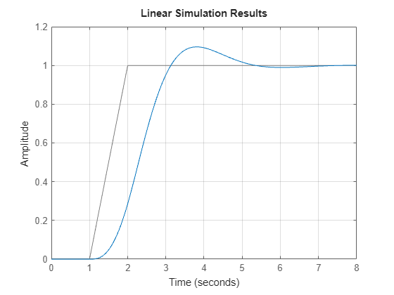
The plot shows the applied input (u,t) in gray and the system response in blue.
Modify the chart object to change the time units to minutes.
lp.TimeUnit = "minutes";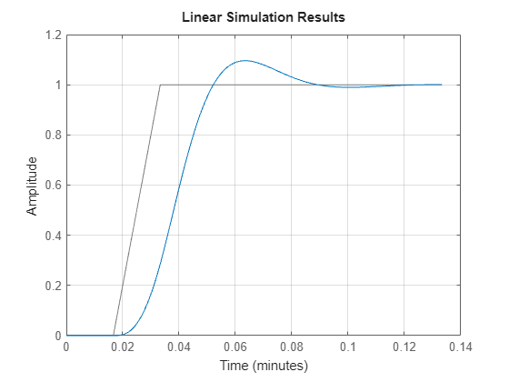
The plot automatically updates when you modify the chart object.
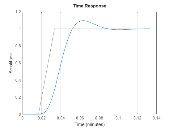
Alternatively, you can also use the timeoptions command to specify the required plot options. First, create an options set based on the toolbox preferences.
plotoptions = timeoptions('cstprefs');Change properties of the options set by setting the time units to minutes and enabling the grid.
plotoptions.TimeUnits = 'minutes';
plotoptions.Grid = 'on';
lsimplot(sys,u,t,plotoptions);
lsimplot allows you to plot the simulated responses of multiple dynamic systems on the same axis. For instance, compare the closed-loop response of a system with a PI controller and a PID controller. Then, customize the plot by enabling normalization and turning the grid on.
First, create a transfer function of the system and tune the controllers.
H = tf(4,[1 10 25]);
C1 = pidtune(H,'PI');
C2 = pidtune(H,'PID');
Form the closed-loop systems.
sys1 = feedback(H*C1,1);
sys2 = feedback(H*C2,1);
Plot the responses of both systems to a square wave with a period of 4 s.
[u,t] = gensig("square",4,12);
lp1 = lsimplot(sys1,sys2,u,t);
legend("PI","PID");

Enable normalization and turn on the grid.
lp1.Normalize = "on";
grid on

The plot automatically updates when you modify the chart object properties.
By default, lsimplot chooses distinct colors for each system that you plot. You can specify colors and line styles using the LineSpec input argument. The first LineSpec "r--" specifies a dashed red line for the response with the PI controller. The second LineSpec "b" specifies a solid blue line for the response with the PID controller. The legend reflects the specified colors and line styles.
lp2 = lsimplot(sys1,"r--",sys2,"b",u,t);
legend("PI","PID");
lp2.Normalize = "on";
grid on

By default, lsimplot simulates the model assuming all states are zero at the start of the simulation. When simulating the response of a state-space model, use the optional x0 input argument to specify nonzero initial state values. Consider the following two-state SISO state-space model.
A = [-1.5 -3;
      3   -1];
B = [1.3; 0];
C = [1.15 2.3];
D = 0;
sys = ss(A,B,C,D);
Suppose that you want to allow the system to evolve from a known set of initial states with no input for 2 s, and then apply a unit step change. Specify the vector x0 of initial state values, and create the input vector.
x0 = [-0.2 0.3];
t = 0:0.05:8;
u = zeros(length(t),1);
u(t>=2) = 1;
First, create a default options set using timeoptions.
plotoptions = timeoptions;
Next change the required properties of the options set plotoptions and plot the simulated response with the zero order hold option.
plotoptions.Title.FontSize = 15;
plotoptions.Title.Color = [0 0 1];
plotoptions.Grid = 'on';
h = lsimplot(sys,u,t,x0,plotoptions,'zoh');
hold on
title('Simulated Time Response with Initial Conditions')
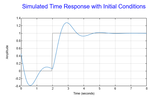
The first half of the plot shows the free evolution of the system from the initial state values [-0.2 0.3]. At t = 2 there is a step change to the input, and the plot shows the system response to this new signal beginning from the state values at that time. Because plotoptions begins with a fixed set of options, the plot result is independent of the toolbox preferences of the MATLAB session.
Since R2025a
Create a state-space model with complex coefficients.
A = [-2-2i -2;1 0];
B = [2;0];
C = [0 0.5+2.5i];
D = 0;
sys = ss(A,B,C,D);
Plot the response of the system to a square wave with a period of 4 s.
[u,t] = gensig("square",4,12);
lp = lsimplot(sys,u,t);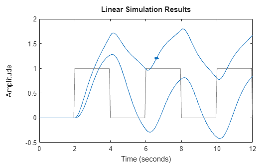
By default, the plot shows the real and imaginary components of the response on a single axes, indicating the imaginary component using a diamond marker.
You can also view the complex response using either a magnitude-phase plot or a complex-plane plot. For example, to view the magnitude and phase of the response, right-click the plot area and select Complex View >Magnitude-Phase.
Alternatively, you can set the ComplexViewType parameter of the corresponding chart object.
lp.ComplexViewType = "magnitudephase";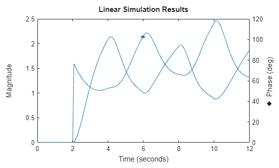
The plot shows the magnitude and phase of the response on a single axes, indicating the phase plot using a diamond marker.
You can view response characteristics in the plot. For example, to view the peak response, right-click the plot and select Characteristics > Peak Response.
Alternatively, you can enable the Visible property of the corresponding characteristic parameter of the chart object.
lp.Characteristics.PeakResponse.Visible = "on";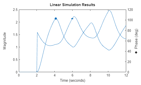
Tips
Plots created using
lsimplotdo not support multiline titles or labels specified as string arrays or cell arrays of character vectors. To specify multiline titles and labels, use a single string with anewlinecharacter.lsimplot(sys,u,t) title("first line" + newline + "second line");
Version History
Introduced in R2012aSee Also
Topics
- Customize Linear Analysis Plots at Command Line (Control System Toolbox)
- Working with the Linear Simulation Tool (Control System Toolbox)