Detect Risk Trees Near Power Lines
This example shows how to detect trees that could fall on power lines and cause outages and interruptions. Risk trees are detected from point clouds collected from Aerial Lidar Scanning (ALS). Lidar can provide information on the vertical structure of the trees, and can also penetrate foliage to provide the elevation information of the ground. This makes it more suitable for such an analysis as compared to image sensors, such as cameras, or hyperspectral or multispectral image data. With lidar-based risk tree detection, utility companies can predict vegetation-related power outages and take preventative measures, as well as more efficiently restore power.
This example also shows how to visualize a risk tree distribution on a map, helping to analyze risk on a geospatial scale.
Load Point Cloud
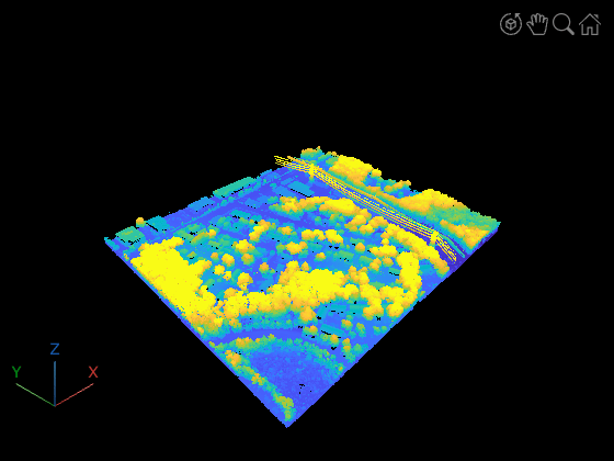
Load a point cloud from a LAZ file using lasFileReader. This file was obtained from the U.S. Geological Survey (USGS) 3DEP LidarExplorer [1], which contains point clouds for various regions of United States. To download a different file, while viewing the 3DEP LidarExplorer map, hold Ctrl and drag to draw a rectangular area of interest.
% Read point cloud from LAZ file
fileName = matlab.internal.examples.downloadSupportFile("lidar","data/ma2021_cent_east.laz");
lasReader = lasFileReader(fileName);
fullPointCloud = readPointCloud(lasReader);

% Visualize
pcviewer(fullPointCloud);
Extract Power Lines
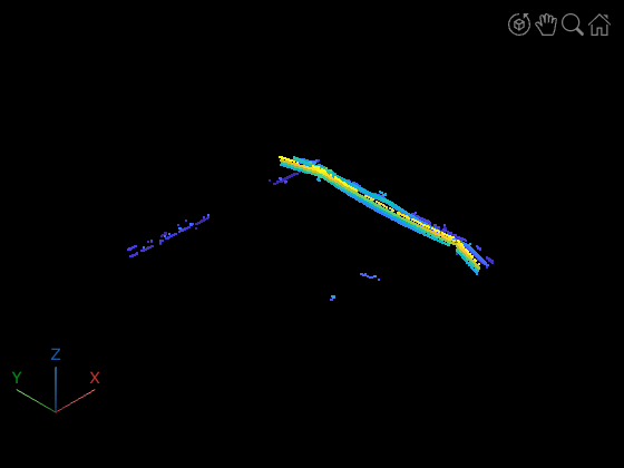
To analyze the risk trees, you must determine the locations of power lines. Extract the power lines from the point cloud using the RandLA-Net (randlanet) deep learning network to perform semantic segmentation. This example uses a pretrained network, trained on the DALES data set [2].
% Create a pretrained RandLA-Net
segmenter = randlanet("dales");

% Downsample point cloud for faster processing. You can skip this
% step to segment the full point cloud and obtain even more precise results.
ptCloud = pcdownsample(fullPointCloud,"gridNearest",0.5);

% Perform inference to predict labels.
labels = segmentObjects(segmenter,ptCloud);

% Extract power lines
fullPowerlinesPtCloud = select(ptCloud,labels == "powerlines");

% Remove noise in segmented point cloud
powerlinesPtCloud = pcdenoise(fullPowerlinesPtCloud,NumNeighbors=40);

% Visualize
pcviewer(powerlinesPtCloud);
Segment Individual Trees
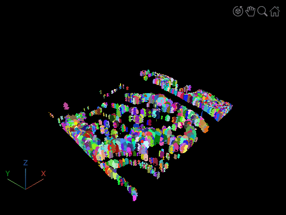
Segmentation of each tree in the point cloud helps analyze whether each tree poses a risk. Extract all the vegetation points from the output labels.
vegetationPtCloud = select(ptCloud,labels == "vegetation");The Extract Individual Tree Attributes and Forest Metrics from Aerial Lidar Data example shows how to segment individual trees from point cloud data by applying image processing techniques to a canopy height model (CHM). CHMs are raster representations of the heights of trees, buildings, and other structures above ground. Use marker-controlled watershed segmentation is to segment individual trees. You can convert the obtained 2-D labels to 3-D, since this data was collected from an aerial vehicle.
% Set minTreeHeight to 10 m. Any vegetation below 10 m is not
% considered for tree segmentation.
minTreeHeight = 10;

label3D = helperSegmentIndividualTrees(ptCloud, vegetationPtCloud, minTreeHeight);
Detect Risk Trees
With the locations of the power lines and the individual trees, you can identify the risk trees. If the height of the tree is greater than d, where d is the distance from the powerline to the bottom of the tree*,* then classify it as a risk tree [3][5].

To calculate d, use the closest power line point to the bottom of a tree apex and bottom locations of the tree.
uniqueLabels = unique(label3D);

% All the tree points have a label value > 0.
uniqueLabels = uniqueLabels(2:end);
numTrees = numel(uniqueLabels);

riskTreeIndices = false(ptCloud.Count,1);

for treeIdx = 1:numTrees
    treePointIndices = (label3D==treeIdx);
    treePoints = ptCloud.Location(treePointIndices,:);
    [treeApexHeight,treeApexPtId] = max(treePoints(:,3));
    [treeBottomHeight,treeBottomPtId] = min(treePoints(:,3));

    % Find nearest power line point to tree bottom point
    treeLocationXY = [treePoints(treeBottomPtId,1) treePoints(treeBottomPtId,2)];
    k = dsearchn(powerlinesPtCloud.Location(:,1:2),treeLocationXY);

    % Calculate d
    distance = norm(powerlinesPtCloud.Location(k,:) - treePoints(treeBottomPtId,:));

    treeHeight = treeApexHeight - treeBottomHeight;

    % Classify risk trees
    if treeHeight > distance

        riskTreeIndices(treePointIndices) = true;

    end
end
Since the point cloud data consists of fully specified 3-D points, all the required information had already been calculated, and you do not require any additional location information for the power lines to determine their heights or their proximity to trees.
Visualize Risk Trees on Map
Visualizing risk trees on a map helps to perform power-line-related vegetation management on a large scale [4]. To visualize the results, you must convert point cloud locations to geographical coordinates (latitude, longitude). Extract the coordinate reference system (CRS) from the LAZ file by using the readCRS function. The CRS information consists of a geographic CRS and several parameters used to transform coordinates to and from the geographic CRS.
% Read the CRS
projCRS = readCRS(lasReader);
Convert the point cloud from Cartesian coordinates to geographic coordinates using the projinv function.
% Convert the point cloud x- and y-coordinates to latitude and longitude
[lat,lon] = projinv(projCRS,ptCloud.Location(:,1), ptCloud.Location(:,2));
Visualize the power lines, risk trees, and safe trees on a 2-D map using the geoplot (Mapping Toolbox) function.
% Visualize on a 2-D map
powerlineIndices = (labels == "powerlines");
nonRiskTreeIndices = (label3D > 0 & ~riskTreeIndices);

figure
% Non-risk trees
geoplot(lat(nonRiskTreeIndices),lon(nonRiskTreeIndices),LineStyle="none",Marker=".",MarkerEdgeColor="green",MarkerSize=1)

% Risk trees
hold on
geoplot(lat(riskTreeIndices),lon(riskTreeIndices),LineStyle="none",Marker=".",MarkerEdgeColor="red",MarkerSize=2)

% Power lines
hold on
geoplot(lat(powerlineIndices),lon(powerlineIndices),LineStyle="none",Marker=".",MarkerEdgeColor="magenta",MarkerSize=4)

hold off
geobasemap satellite
legend("Safe Trees", "Risk Trees", "Powerlines")

Visualize the risk plot on a 3-D geographic globe by using the geoglobe (Mapping Toolbox) function.
% Extract the heights of the points
altitude = ptCloud.Location(:,3);

g = geoglobe(uifigure);
geoplot3(g, lat(powerlineIndices),lon(powerlineIndices),altitude(powerlineIndices),"mo", MarkerSize=0.5)

hold(g,"on")
geoplot3(g, lat(riskTreeIndices),lon(riskTreeIndices),altitude(riskTreeIndices),"ro", MarkerSize=0.5)
geoplot3(g, lat(nonRiskTreeIndices),lon(nonRiskTreeIndices),altitude(nonRiskTreeIndices),"go",MarkerSize=0.5)
hold(g,"off")

% Set the camera height
camheight(g,5*max(altitude))

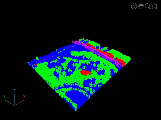
Visualize the risk trees in the point cloud.
% Set color for each point in point cloud

color = repmat([0 0 1],ptCloud.Count,1); % Blue
color(powerlineIndices,:) = repmat([1 0 1],nnz(powerlineIndices),1); % Magenta - Powerlines
color(nonRiskTreeIndices,:) = repmat([0 1 0],nnz(nonRiskTreeIndices),1); % Green - Safe trees
color(riskTreeIndices,:) = repmat([1 0 0],nnz(riskTreeIndices),1); % Red - Risk trees

pcviewer(ptCloud,color);
References
[1] U.S. Geological Survey (USGS). 3DEP LidarExplorer https://apps.nationalmap.gov/lidar-explorer/.
[2] Varney, Nina, Vijayan K. Asari, and Quinn Graehling. “DALES: A Large-Scale Aerial LiDAR Data Set for Semantic Segmentation.” In 2020 IEEE/CVF Conference on Computer Vision and Pattern Recognition Workshops (CVPRW), 717–26. Seattle, WA, USA: IEEE, 2020. https://doi.org/10.1109/CVPRW50498.2020.00101.
[3] Wedegedara, H., C. Witharana, D. Joshi, D. Cerrai, and R. Fahey. "Geospatial Modeling of Roadside Vegetation Risk on Distribution Power Lines in Connecticut", The International Archives of the Photogrammetry, Remote Sensing and Spatial Information Sciences, XLVI-M-2-2022, (July 25, 2022): 217–24. https://doi.org/10.5194/isprs-archives-XLVI-M-2-2022-217-2022.
[4] Hartling, Sean, Vasit Sagan, Maitiniyazi Maimaitijiang, William Dannevik, and Robert Pasken. "Estimating Tree-Related Power Outages for Regional Utility Network Using Airborne LiDAR Data and Spatial Statistics." International Journal of Applied Earth Observation and Geoinformation 100 (August 2021): 102330. https://doi.org/10.1016/j.jag.2021.102330.
[5] Wanik, D.W., J.R. Parent, E.N. Anagnostou, and B.M. Hartman. "Using Vegetation Management and LiDAR-Derived Tree Height Data to Improve Outage Predictions for Electric Utilities." Electric Power Systems Research 146 (May 2017): 236–45. https://doi.org/10.1016/j.epsr.2017.01.039.