imshow

Display image

Syntax

imshow(I)

imshow(I,[low high])

imshow(I,[])

imshow(RGB)

imshow(BW)

imshow(X,map)

imshow(filename)

imshow(___,Name,Value)

himage = imshow(___)

Description

imshow(I) displays the grayscale image I in a figure. imshow uses the default display range for the image data type and optimizes figure, axes, and image object properties for image display.

imshow(I,[low high]) displays the grayscale image I, specifying the display range as a two-element vector, [low high]. For more information, see the DisplayRange argument.

imshow(I,[]) displays the grayscale image I, scaling the display based on the range of pixel values in I. imshow uses [min(I(:)) max(I(:))] as the display range. imshow displays the minimum value in I as black and the maximum value as white. For more information, see the DisplayRange argument.

imshow(RGB) displays the truecolor image RGB in a figure.

imshow(BW) displays the binary image BW in a figure. For binary images, imshow displays pixels with the value 0 (zero) as black and 1 as white.

imshow(X,map) displays the indexed image X with the colormap map.

imshow(filename) displays the image stored in the graphics file specified by filename.

imshow(___,Name,Value) displays an image, using name-value pairs to control aspects of the operation.

himage = imshow(___) returns the image object created by imshow.

Examples

Display RGB, Grayscale, Binary, or Indexed Image

Display an RGB (truecolor), grayscale, binary, or indexed image using imshow.

Display an RGB Image

Read a sample RGB image, peppers.png, into the MATLAB workspace.

rgbImage = imread("peppers.png");

Display the RGB image using imshow.

imshow(rgbImage)

Display a Grayscale Image

Convert the RGB image to a grayscale image by using the rgb2gray function.

grayImage = rgb2gray(rgbImage);

Display the grayscale image using imshow.

imshow(grayImage)

Display a Binary Image

Convert the grayscale image to a binary image by using thresholding.

meanVal = mean(grayImage,"all");
binaryImage = grayImage >= meanVal;

Display the binary image using imshow.

imshow(binaryImage)

Display an Indexed Image

Read a sample indexed image, corn.tif, into the MATLAB workspace.

[corn_indexed,map] = imread('corn.tif');

Display the indexed image using imshow.

imshow(corn_indexed,map)

Display Image from File

Display an image stored in a file.

imshow('peppers.png');

Change Colormap of Displayed Image

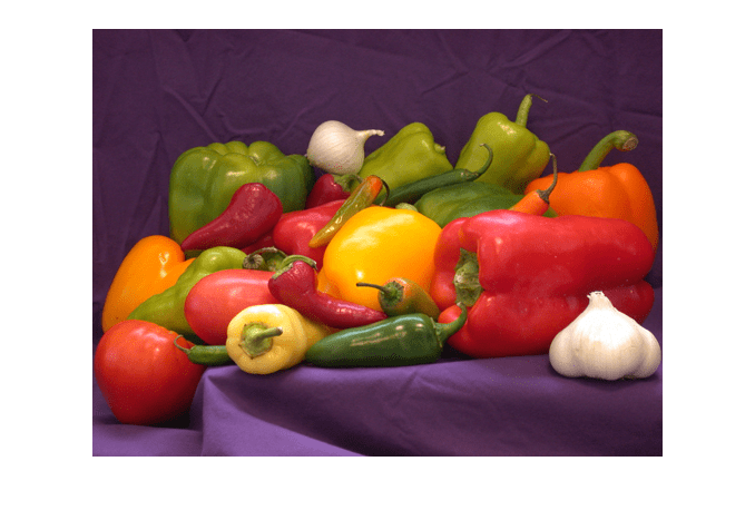
Load a sample grayscale volumetric image, mri.mat, into the variable D in the workspace. Remove the singleton dimension of the volume using the squeeze function.

load("mri.mat");
vol = squeeze(D);

Select a slice from the middle of the volume. Display the slice using the copper colormap and scaling the display range to the range of pixel values.

sliceZ = vol(:,:,13);
imshow(sliceZ,[],Colormap=copper)

Change the colormap for the image using the colormap function.

colormap(hot)

Scale Display Range of Image

Read a truecolor (RGB) image into the workspace. The data type of the image is uint8.

RGB = imread('peppers.png');

Extract the green channel of the image. The green channel is the second color plane.

G = RGB(:,:,2);
imshow(G)

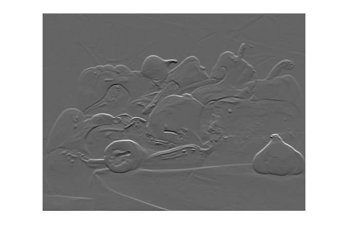
Create a filter that detects horizontal edges in the image.

filt = [-1 -1 -1;0 0 0;1 1 1];

Filter the green channel of the image using the filter2 function. The result is an image of data type double, with a minimum value of -422 and a maximum value of 656. Pixels with a large magnitude in the filtered image indicate strong edges.

edgeG = filter2(filt,G);

Display the filtered image using imshow with the default display range. For images of data type double, the default display range is [0, 1]. The image appears black and white because the filtered pixel values exceed the range [0, 1].

imshow(edgeG)

Display the filtered image and scale the display range to the pixel values in the image. The image displays with the full range of grayscale values.

imshow(edgeG,[])

Magnify Image using Nearest Neighbor and Bilinear Interpolation

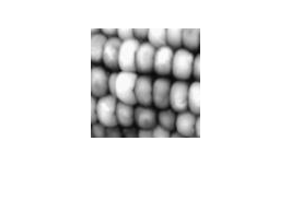
Read the grayscale image from the corn.tif file into the workspace. The grayscale version of the image is the second image in the file.

corn_gray = imread('corn.tif',2);

Select a small portion of the image. Display the detail image at 100% magnification using imshow.

corn_detail = corn_gray(1:100,1:100);
imshow(corn_detail)

Display the image at 1000% magnification by using the 'InitialMagnification' name-value pair argument. By default, inshow performs nearest neighbor interpolation of pixel values. The image has blocking artifacts.

imshow(corn_detail,'InitialMagnification',1000)

Display the image at 1000% magnification, specifying the bilinear interpolation technique. The image appears smoother.

imshow(corn_detail,'InitialMagnification',1000,'Interpolation',"bilinear")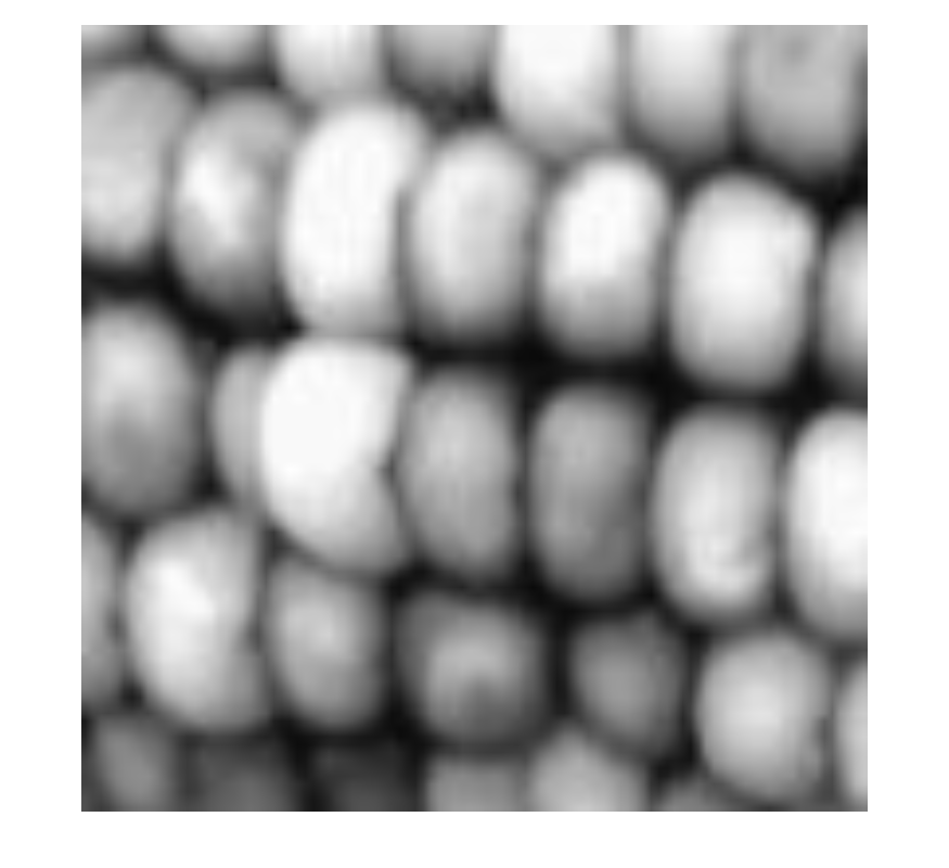

Input Arguments

I — Input grayscale image

matrix

Input grayscale image, specified as a matrix. A grayscale image can be any numeric data type.

Data Types: single | double | int8 | int16 | int32 | int64 | uint8 | uint16 | uint32 | uint64 | logical

RGB — Input truecolor image

m-by-n-by-3 array

Input truecolor image, specified as an m-by-n-by-3 array.

If you specify a truecolor image of data type single or double, then values should be in the range [0, 1]. If pixel values are outside this range, then you can use the rescale function to scale pixel values to the range [0, 1]. The 'DisplayRange' argument has no effect when the input image is truecolor.

Data Types: single | double | uint8 | uint16

BW — Input binary image

matrix

Input binary image, specified as a matrix.

Data Types: logical

X — Indexed image

2-D matrix of positive integers

Indexed image, specified as a 2-D matrix of positive integers. The values in X are indices into the colormap specified by map.

Data Types: single | double | uint8 | logical

map — Colormap

c-by-3 matrix

Colormap associated with indexed image X, specified as a c-by-3 matrix. Each row of map is a three-element RGB triplet that specifies the red, green, and blue components of a single color of the colormap. When map is of data type single or double, the values of the matrix are in the range [0, 1].

Data Types: single | double | uint8

filename — File name

character vector

File name, specified as a character vector. The image must be readable by the imread function. The imshow function displays the image, but does not store the image data in the MATLAB^® workspace. If the file contains multiple images, then imshow displays the first image in the file.

Example: 'peppers.png'

Data Types: char

[low high] — Grayscale image display range

two-element vector

Grayscale image display range, specified as a two-element vector. For more information, see the 'DisplayRange' name-value pair argument.

Example: [50 250]

Data Types: single | double | int8 | int16 | int32 | int64 | uint8 | uint16 | uint32 | uint64

Name-Value Arguments

Specify optional pairs of arguments as Name1=Value1,...,NameN=ValueN, where Name is the argument name and Value is the corresponding value. Name-value arguments must appear after other arguments, but the order of the pairs does not matter.

Before R2021a, use commas to separate each name and value, and enclose Name in quotes.

Example: imshow('board.tif','Border','tight')

Border — Figure window border space

'loose' (default) | 'tight'

Figure window border space, specified as the comma-separated pair consisting of 'Border' and either 'tight' or 'loose'. When set to 'loose', the figure window includes space around the image in the figure. When set to 'tight', the figure window does not include any space around the image in the figure.

If the image is very small or if the figure contains other objects besides an image and its axes, imshow might use a border regardless of how this parameter is set.

Data Types: char

Colormap — Colormap

c-by-3 matrix

Colormap of the axes, specified as the comma-separated pair consisting of 'Colormap' and a c-by-3 matrix with values in the range [0, 1]. Each row of the matrix is a three-element RGB triplet that specifies the red, green, and blue components of a single color of the colormap. Use this argument to view grayscale images in false color. If you specify an empty colormap ([]), then the imshow function ignores this argument.

Example: cmap = copper; imshow('board.tif','Colormap',cmap)

Data Types: double

DisplayRange — Grayscale image display range

two-element vector | []

Display range of a grayscale image, specified as a two-element vector of the form [low high]. The imshow function displays the value low (and any value less than low) as black, and it displays the value high (and any value greater than high) as white. Values between low and high are displayed as intermediate shades of gray, using the default number of gray levels.

If you specify an empty matrix ([]), then imshow uses a display range of [min(I(:)) max(I(:))]. In other words, the minimum value in I is black, and the maximum value is white.

If you do not specify a display range, then imshow selects a default display range based on the image data type.

• If I is an integer type, then DisplayRange defaults to the minimum and maximum representable values for that integer class. For example, the default display range for uint16 arrays is [0, 65535].

• If I is data type single or double, then the default display range is [0, 1].

Note

Including the parameter name is optional, except when the image is specified by a file name. The syntax imshow(I,[low high]) is equivalent to imshow(I,'DisplayRange',[low high]). If you call imshow with a file name, then you must specify the 'DisplayRange' parameter.

Example: 'DisplayRange',[10 250]

Data Types: single | double | int8 | int16 | int32 | int64 | uint8 | uint16 | uint32 | uint64

InitialMagnification — Initial magnification of image display

100 (default) | numeric scalar | 'fit'

Initial magnification of the image display, specified as the comma-separated pair consisting of 'InitialMagnification' and a numeric scalar or 'fit'. If set to 100, then imshow displays the image at 100% magnification (one screen pixel for each image pixel). If set to 'fit', then imshow scales the entire image to fit in the window.

Initially, imshow attempts to display the entire image at the specified magnification. If the magnification value is so large that the image is too big to display on the screen, imshow displays the image at the largest magnification that fits on the screen.

If the image is displayed in a figure with its 'WindowStyle' property set to 'docked', then imshow displays the image at the largest magnification that fits in the figure.

Note: If you specify the axes position, imshow ignores any initial magnification you might have specified and defaults to the 'fit' behavior.

When you use imshow with the 'Reduce' parameter, the initial magnification must be 'fit'.

In MATLAB Online™, 'InitialMagnification' is set to 'fit' and cannot be changed.

Example: 'InitialMagnification',80

Data Types: single | double | int8 | int16 | int32 | int64 | uint8 | uint16 | uint32 | uint64 | char

Interpolation — Interpolation technique

'nearest' (default) | 'bilinear'

Interpolation method, specified as 'nearest' or 'bilinear'. MATLAB uses interpolation to display a scaled version of the image on your screen. The value you choose does not affect the image data. Choose an interpolation method based on your image content and the effect you want to achieve:

• 'nearest' — Nearest neighbor interpolation. The value of a pixel located at (x, y) is the value of the pixel that is closest to (x, y) in the original image. This method is best when there are a small number of pixel values that represent distinct categories, or when you want to see individual pixels in a highly zoomed-in view.

• 'bilinear' — Bilinear interpolation. The value of a pixel located at (x, y) is a weighted average of the surrounding pixels in the original image. To minimize display artifacts, the imshow function performs antialiasing when you shrink the image. This method is best in almost all other situations.

Parent — Parent axes of image object

Axes object | UIAxes object

Parent axes of image object, specified as the comma-separated pair consisting of 'Parent' and an Axes object or a UIAxes object. Use the 'Parent' name-value argument to build a UI that gives you control of the Figure and Axes properties.

Reduce — Indicator for subsampling

true | false | 1 | 0

Indicator for subsampling image, specified as the comma-separated pair consisting of 'Reduce' and either true, false, 1, or 0. This argument is valid only when you use it with the name of a TIFF file. Use the Reduce argument to display overviews of very large images.

Data Types: logical

XData — X-axis limits of nondefault coordinate system

two-element vector

X-axis limits of nondefault coordinate system, specified as the comma-separated pair consisting of 'XData' and a two-element vector. This argument establishes a nondefault spatial coordinate system by specifying the image XData. The value can have more than two elements, but imshow uses only the first and last elements.

Example: 'XData',[100 200]

Data Types: single | double | int8 | int16 | int32 | int64 | uint8 | uint16 | uint32 | uint64

YData — Y-axis limits of nondefault coordinate system

two-element vector

Y-axis limits of nondefault coordinate system, specified as the comma-separated pair consisting of 'YData' and a two-element vector. The value can have more than two elements, but imshow uses only the first and last elements.

Example: 'YData',[100 200]

Data Types: single | double | int8 | int16 | int32 | int64 | uint8 | uint16 | uint32 | uint64

Output Arguments

himage — Image created by imshow

image object

Image created by the imshow function, specified as an image object.

Tips

• To change the colormap after you create the image, use the colormap command.

• You can display multiple images with different colormaps in the same figure using imshow with the tiledlayout and nexttile functions.

• You can create an axes on top of the axes created by imshow by using the hold on command after calling imshow.

• The imshow function is not supported when you start MATLAB with the -nojvm option.

• Figure titles can appear cut off in the Live Editor. To ensure the whole title is visible, set the PositionContraint property of the parent axes object to "outerposition". Update the property value after the imshow function and before the title function.

  I = imread("peppers.png");
  imshow(I)
  ax = gca;
  ax.PositionConstraint = "outerposition";
  title("Peppers");

  If you specify the parent axes using the Parent name-value argument, set the PositionConstraint property of the specified parent axes object. For more details about axes position properties, see Control Axes Layout.

Extended Capabilities

GPU Arrays

Accelerate code by running on a graphics processing unit (GPU) using Parallel Computing Toolbox™.

Usage notes and limitations:

• This function accepts GPU arrays, but does not run on a GPU.

For more information, see Run MATLAB Functions on a GPU (Parallel Computing Toolbox).

Distributed Arrays

Partition large arrays across the combined memory of your cluster using Parallel Computing Toolbox™.

Usage notes and limitations:

• This function operates on distributed arrays, but executes in the client MATLAB.

For more information, see Run MATLAB Functions with Distributed Arrays (Parallel Computing Toolbox).

Version History

Introduced before R2006a