Optimizing Normalizer Breakpoints and Table Values
Optimizing breakpoints alters the position of the table normalizers so that the total square error between the model and the table is reduced.
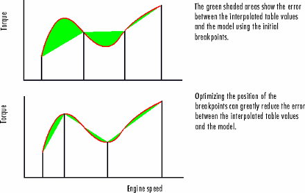
This routine improves the fit between your strategy and your model. The following illustration shows how the optimization of breakpoint positions can reduce the difference between the model and the table. The breakpoints are moved to reduce the peak error between breakpoints. In CAGE this happens in two dimensions across a table.
Filling Methods
The methods for spacing the breakpoints of your normalizers in CAGE are:
For one-dimensional tables
ReduceErrorShareAveCurv
For two-dimensional tables
ShareAveCurvShareCurvThenAve
ReduceError
Spacing breakpoints using ReduceError uses a greedy algorithm. CAGE:
Locks two breakpoints at the extremities of the range of values.
Interpolates the function between these two breakpoints.
Calculates the maximum error between the model and the interpolated function.
Places a breakpoint where the error is maximum.
Repeats steps 2, 3, and 4.
Locates all the breakpoints, ending the algorithm.
ShareAveCurv and ShareCurvThenAve
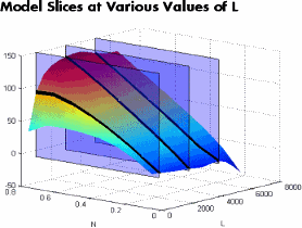
Consider calibrating the normalizers for speed, N, and relative air-charge, L, in the preceding MBT model.
In both cases, CAGE approximates the MBTAV(N, L) model, in this case, using a fine mesh.
The breakpoints of each normalizer are calibrated in turn. In this example, these routines calibrate the normalizer in N first.
Spacing breakpoints using ShareAveCurv or
ShareCurvThenAve calculates the curvature,
K, of the model
MBTAV(N, L):
![]()
as an approximation for
![]()
Both routines calculate the curvature for a number of slices of the model at various values of L. For example, the figure shown has a number of slices of a model at various values of L.
ShareAveCurvaverages the curvature over the range of L, then spaces the breakpoints by placing the ith breakpoint according to the following rule.ShareCurvThenAveplaces the ith breakpoint according to the rule, then finds the average position of each breakpoint.
Rule for Placing Breakpoints
If j breakpoints need to be placed, the ith breakpoint, Ni, is placed where the average curvature is[1]:
![]()
This condition spaces out the breakpoints so that an equal amount of curvature (in an appropriate metric) occurs in each breakpoint interval. The breakpoint placement is optimal in the sense that the maximum error between the lookup table estimate and the model decreases with the optimal convergence rate of O(N-2). For reference, consider that equally spaced breakpoints have an order of O(N-1/2).
Optimizing Table Values
The Feature Fill Wizard optimizes the table values to minimize the current total square error between the feature values and the model.
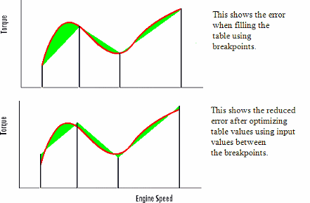
This routine optimizes the fit between your strategy and your model. Using Fill places values into your table. The optimization process shifts the cell values up and down to minimize the overall error between the interpolation between the model and the strategy.
In this example, the green shaded areas show the error between the mesh model (evaluated at the number of grid points you choose) and the table values.
CAGE evaluates the model over the number of grid points specified in the Feature Fill
Wizard, then calculates the total square error between this mesh model and the feature
values. CAGE adjusts the table values until this error is minimized, using
lsqnonlin if there are no gradient constraints. Otherwise, CAGE
uses fmincon with linear constraints to specify the gradient of the
table at each cell.
References
[1] Boor, Carl de. A Practical Guide to Splines. New York: Springer-Verlag, 1978, pp 46.