Run Field Oriented Control of PMSM Using Model Predictive Control
This example uses Model Predictive Control (MPC) to control the speed of a three-phase permanent magnet synchronous motor (PMSM).
MPC involves solving plant equations to find the sequence of inputs that minimize a cost function over a finite, receding, horizon. The first control action of the sequence is applied and then the process is repeated at the each time step.


The optimizer provides the optimal inputs to the model based on solving the objective function under specific bounds and constraints. During Prediction step, the future response of a plant is predicted with the help of a dynamic discrete-time model up to  sampling intervals, which is called the prediction horizon. During Optimization step, the objective function is solved to obtain the optimal control inputs up to
  sampling intervals, which is called control horizon for the predicted response. Control horizon remains less than or equal to the prediction horizon.

The example uses an MPC controller as a speed controller (in a field-oriented control or FOC algorithm) with  as the manipulated variable,
  as the measured output, and the load torque
  (estimated using an observer) as the measured disturbance.
The objective function is derived as a linear sum of these:
[W1 * (error in output)] + [W2 * (rate of change of input)]
where, W1, and W2 are the weights.
The example uses the model initialization script to define these weights of these three parameters.
1. Rate of change of input: 
2. Measured Outputs: 
Therefore, by default, the example gives maximum weightage to the output variables parameter (corresponding to ) when calculating the error in the predicted output. You can change the weightage values for error computation using the model initialization script available in the example.
The example also operates the MPC input and the output under the following lower and upper bounds:
Inputs
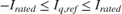
Input rate of change
Measured outputs
 (rad/s)
Additionally, the MPC Controller is this example is configured to used signal previewing (look-ahead). By providing the MPC with a preview of the future speed reference instead of a single value, you can further improve the tacking performance. The example uses a vector of upcoming reference points (total 3 samples) and enables the controller to anticipate reference changes, resulting in smoother torque commands, better tracking during ramps, and improved dynamic response compared to assuming the reference remains constant over the prediction horizon. This is useful for applications where the path or speed reference trajectory is predefined.
For more information about MPC, see What Is Model Predictive Control? (Model Predictive Control Toolbox).
Models
The example includes the model SpeedControlofPMSMusingMPC
You can use these models for both simulation and code generation.

For the model names that you can use for different hardware configurations, see the Required Hardware topic in the Generate Code and Deploy Model to Target Hardware section.
Required MathWorks Products
To simulate model:
Motor Control Blockset™
Model Predictive Control Toolbox™
To generate code and deploy model:
Motor Control Blockset
Model Predictive Control Toolbox
Embedded Coder®
C2000™ Microcontroller Blockset
Prerequisites
1. Obtain the motor parameters. We provide default motor parameters with the Simulink® model that you can replace with the values from either the motor datasheet or other sources.
However, if you have the motor control hardware, you can estimate the parameters for the motor that you want to use, by using the Motor Control Blockset parameter estimation tool. For instructions, see Estimate Motor Parameters Using Motor Control Blockset Parameter Estimation Tool.
The parameter estimation tool updates the motorParam variable (in the MATLAB® workspace) with the estimated motor parameters.
2. If you obtain the motor parameters from the datasheet or other sources, update the motor parameters and inverter parameters in the model initialization script associated with the Simulink® models. For instructions, see Estimate Control Gains and Tune Control Parameters.
If you use the parameter estimation tool, you can update the inverter parameters, but do not update the motor parameters in the model initialization script. The script automatically extracts motor parameters from the updated motorParam workspace variable.
Simulate Model
This example supports simulation. Follow these steps to simulate the model.
1. Open a model included with this example.
2. Click Run on the Simulation tab to simulate the model.
3. Click Data Inspector on the Simulation tab to view and analyze the simulation results.
Generate Code and Deploy Model to Target Hardware
This section instructs you to generate code and run the FOC algorithm on the target hardware.
This example uses a host and a target model. The host model is a user interface to the controller hardware board. You can run the host model on the host computer. The prerequisite to use the host model is to deploy the target model to the controller hardware board. The host model uses serial communication to command the target Simulink® model and run the motor in a closed-loop control.
Required Hardware
This example supports this hardware configuration. You can also use the target model name to open the model for the corresponding hardware configuration, from the MATLAB® command prompt.
LAUNCHXL-F28379D controller + BOOSTXL-DRV8305 inverter:
SpeedControlofPMSMusingMPC
For connections related to the preceding hardware configurations, see LAUNCHXL-F28069M and LAUNCHXL-F28379D Configurations.
Generate Code and Run Model on Target Hardware
1. Simulate the target model and observe the simulation results.
2. Complete the hardware connections.
3. The model automatically computes the ADC (or current) offset values. To disable this functionality (enabled by default), update the value 0 to the variable inverter.ADCOffsetCalibEnable in the model initialization script.
Alternatively, you can compute the ADC offset values and update it manually in the model initialization scripts. For instructions, see Run 3-Phase AC Motors in Open-Loop Control and Calibrate ADC Offset.
4. Compute the quadrature encoder index offset value and update it in the model initialization scripts associated with the target model. For instructions, see Quadrature Encoder Offset Calibration for PMSM.
NOTE: Verify the number of slits available in the quadrature encoder sensor attached to your motor. Check and update the variable pmsm.QEPSlits available in the model initialization script. This variable corresponds to the Encoder slits parameter of the quadrature encoder block. For more details about the Encoder slits and Encoder counts per slit parameters, see Quadrature Decoder.
5. Open the target model for the hardware configuration that you want to use. If you want to change the default hardware configuration settings for the model, see Model Configuration Parameters.
6. Load a sample program to CPU2 of LAUNCHXL-F28379D, for example, program that operates the CPU2 blue LED by using GPIO31 (c28379D_cpu2_blink.slx), to ensure that CPU2 is not mistakenly configured to use the board peripherals intended for CPU1. For more information about the sample program or model, see the Task 2 - Create, Configure and Run the Model for TI Delfino F28379D LaunchPad (Dual Core) section in Getting Started with Texas Instruments C2000 Microcontroller Blockset (C2000 Microcontroller Blockset).
7. Click Build, Deploy & Start on the Hardware tab to deploy the target model to the hardware.
8. Click the SpeedControlofPMSMusingMPCHost.slx host model hyperlink in the target model to open the associated host model.

For details about the serial communication between the host and target models, see Host-Target Communication.
9. In the model initialization script associated with the target model, specify the communication port using the variable target.comport. The example uses this variable to update the Port parameter of the Host Serial Setup, Host Serial Receive, and Host Serial Transmit blocks available in the host model.
10. Update the Reference Speed value in the host model.
11. Click Run on the Simulation tab to run the host model.
12. Change the position of the Start / Stop Motor switch to On, to start running the motor.
13. Use the Debug signals section to select the debug signals that you want to monitor. Observe the debug signals from the RX subsystem, in the Time Scope of the host model.
Simulation Results
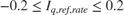
The speed reference profile is shown in the following image.
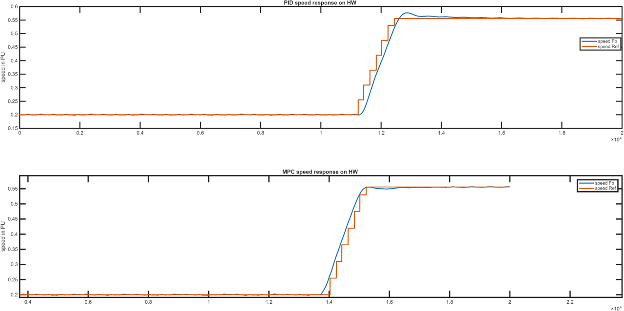
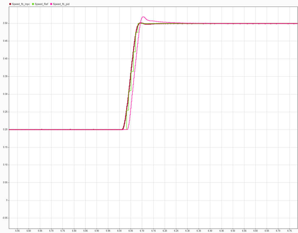
The following image shows a comparison of PID output and MPC output for the speed reference, zoomed around a transition. The MPC controller with a preview of future reference provides a better tracking performance compared to PID, which reacts only after the reference signal changes.
Hardware Results
The above model is tested on Teknik motor with F28379d Launchpad run at 20kHz. The execution time of the speed controller ( MPC + Observer + preemption) is 5e-4 s. Similar to the simulation results, MPC anticipates the changes in the reference signal preemptively and provides a better tracking performance.