Tune PI Controllers (in Field-Weakening Control Mode) Using FOC Autotuner Block
This example uses the Field Oriented Control Autotuner block to compute the gain values of the PI controllers available in the speed, current, and flux control loops of a field-weakening control algorithm. For details about this block, see Field Oriented Control Autotuner.
The example automatically computes the PI controller gains to run an Interior Permanent Magnet Synchronous Motor (IPMSM) using field-weakening control. Field-weakening control is an operating mode that runs the motor at speeds greater than the base speed or rated speed. To enter this mode the example reduces the d-axis stator current ( ) to a negative value, which reduces the rotor flux linkage. This enables the motor to run above the base speed. For more information about this operating mode, see Field-Weakening Control (with MTPA) of PMSM.
Use the code-generation capability of the example to deploy the gain-tuning algorithm to the target hardware. This enables you to run the algorithm on the target hardware connected to a motor and compute accurate PI controller gains by processing motor feedback in real-time on the hardware. The example uses a quadrature encoder sensor to measure the rotor position.
Note: This example provides the field-weakening control algorithm as a reference. You can refer this example and use a similar approach to add the Field Oriented Control Autotuner block and the gain-tuning algorithm to the field-weakening logic available in your model.
Model
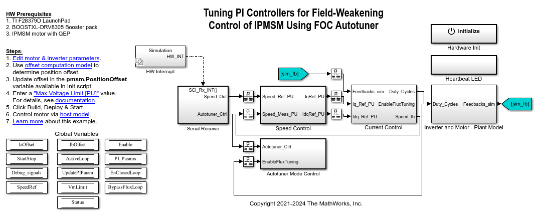
The example includes the target model mcb_ipmsm_fwc_autotuner_f28379d.
You can use this model for both simulation and code generation.
The Field Oriented Control Autotuner block iteratively tunes the d- and q-axis current control, speed and flux control loops and computes the gains of the current, speed, and flux PI controllers. The following figure shows the Field Oriented Control Autotuner block available inside the model:
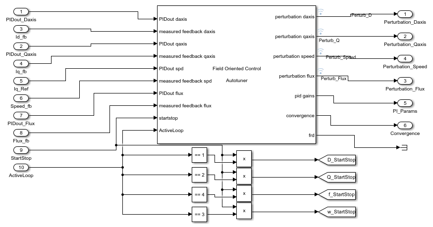
In addition to the current and speed feedback from the plant, the block processes the reference flux and flux feedback values. It also processes the current and speed PI controller outputs to compute the PI controller gains (Kp and Ki).

For more details on the FOC architecture, see Field-Oriented Control.
Required MathWorks Products
To simulate model:
Motor Control Blockset™
Simulink® Control Design™
Stateflow® (needed only if you modify the example model)
To generate code and deploy model:
Motor Control Blockset™
Simulink Control Design™
Embedded Coder®
C2000™ Microcontroller Blockset
Stateflow (needed only if you modify the example model)
Prerequisites for Simulation and Hardware Deployment
1. Open the model initialization script for the target model. Check and update the motor, inverter, and other control system and hardware parameters available in the script. For instructions on locating and editing the model initialization script associated with a target model, see Estimate Control Gains and Tune Control Parameters.
2. In the Inverter & Target Parameters section of the model initialization script, verify that the mcb_SetInverterParameters function uses the argument BoostXL-DRV8305. This enables the script to use the preprogrammed parameters for the BOOSTXL-DRV8305 inverter.
3. Configure these parameters correctly in the model initialization script. These variables are essential for the gain-tuning algorithm to compute the PI controller gains. If the values of these variables are incorrect, the model may fail to bring the motor to the steady speed state.
pmsm.p
pmsm.I_rated
pmsm.PositionOffset
pmsm.QEPSlits
4. If you are using a motor that is not listed in the mcb_SetPMSMMotorParameters function (used in the System Parameters // Hardware parameters section of the model initialization script), tune the default values of the following initial gains available in the Initial PI parameters section of the model initialization script. This ensures that the motor reaches the steady state of speed-control operation:
PI_params.Kp_Id
PI_params.Ki_Id
PI_params.Kp_Iq
PI_params.Ki_Iq
PI_params.Kp_Speed
PI_params.Ki_Speed
PI_params.Kp_Flux
PI_params.Ki_Flux
When you either simulate or run the example on a target hardware, the example uses crude values of the PI controller gains to achieve the steady state of speed-control operation.
Note: When using this example, if the motor (whether it is listed or not in the mcb_SetPMSMMotorParameters function) does not run, try tuning the default values of these parameters.
5. In the FOC Autotuner parameters section of the model initialization script, check and update the parameters of the Field Oriented Control Autotuner block. This sets the reference bandwidth and phase margin values for both the speed and the current PI controllers.
Simulate the Target Model
Simulating the example is optional. Follow these steps to simulate the target model:
1. Open the target model.
2. Click Run on the Simulation tab to simulate the target model.
3. Observe the computed PI controller gain values in the Display blocks available in the mcb_ipmsm_fwc_autotuner_f28379d/Current Control/PI_Params_Display_and_Logging subsystem.
The computed gains might not be accurate because step 3 in the Prerequisites for Simulation and Hardware Deployment section checks the accuracy of only four motor parameters.
If you want to compute and test the PI controller gains using simulation, follow these steps before clicking Run on the Simulation tab of the target model.
In the System Parameters // Hardware parameters section of the model initialization script, verify that the
mcb_SetPMSMMotorParametersfunction uses an argument that represents your motor (for example,Teknic2310P). Open themcb_SetPMSMMotorParametersfunction to see the preprogrammed cases that store the motor parameters of commonly used PMSMs.
If the mcb_SetPMSMMotorParameters function does not list your PMSM, determine the parameters for your motor using these steps.
If you have motor control hardware, you can estimate the parameters for your motor, by using the Motor Control Blockset parameter estimation tool. For instructions, see Estimate Motor Parameters Using Motor Control Blockset Parameter Estimation Tool and Estimate PMSM Parameters Using Custom Hardware.
The parameter estimation tool updates the motorParam variable (in the MATLAB® workspace) with the estimated motor parameters.
If you obtain the motor parameters from the datasheet or other sources, add and configure the motor parameters in the model initialization script. These parameter values override the selected pre-programmed case in the function
mcb_SetPMSMMotorParameters.
If you use the parameter estimation tool, do not update the motor parameters directly in the model initialization script. The script automatically extracts the motor parameters from the updated motorParam variable in the workspace.
After you simulate the target model and determine the gains, update your model (that implements field-weakening control) with the computed gain values to quickly bring the motor to a steady speed state.
Deploy the example to the target hardware to tune the PI controller gains more accurately by using an actual hardware connected to a motor. For more details, see the Generate Code and Deploy Model to Target Hardware section.
Generate Code and Deploy Model to Target Hardware
This section shows how to generate code and run the algorithm for tuning the PI controller gains on the target hardware. Running the example on the hardware enables you to compute the PI controller gains more accurately by processing the feedback from an actual plant in real-time.
This example uses a host and a target model. The host model is a user interface to the controller hardware board. You can run the host model on the host computer. Before you run the host model on the host computer, deploy the target model to the controller hardware board. The host model uses serial communication to command the target model and run the motor in closed-loop control.
Required Hardware
The example supports the following hardware configuration. You can also use the target model name to open the model from the MATLAB® command prompt.
LAUNCHXL-F28379D controller + BOOSTXL-DRV8305 inverter: mcb_ipmsm_fwc_autotuner_f28379d
For more information on connections related to this hardware configuration, see LAUNCHXL-F28069M and LAUNCHXL-F28379D Configurations.
Generate Code and Run Model on Target Hardware
1. Complete the hardware connections.
2. The model automatically computes the analog to digital converter (ADC) offset (also known as current offset). To disable this functionality (enabled by default), update the value of the inverter.ADCOffsetCalibEnable variable in the model initialization script to 0.
Alternatively, you can compute the ADC offset values and update them manually in the model initialization script. For instructions, see Run 3-Phase AC Motors in Open-Loop Control and Calibrate ADC Offset.
3. Compute the quadrature encoder index offset value and update it in the pmsm.PositionOffset variable in the model initialization script of the target model. For instructions, see Quadrature Encoder Offset Calibration for PMSM.
4. Open the target model. If you want to change the default hardware configurations of the model, see Model Configuration Parameters.
5. Load a sample program to the CPU2 of the LAUNCHXL-F28379D board. For example, load the program that operates the CPU2 blue LED by using GPIO31 (c28379D_cpu2_blink.slx). This ensures that CPU2 is not mistakenly configured to use the board peripherals intended for CPU1. For more information about the sample program or model, see the Task 2 - Create, Configure and Run the Model for TI Delfino F28379D LaunchPad (Dual Core) section in Getting Started with Texas Instruments C2000 Microcontroller Blockset (C2000 Microcontroller Blockset).
6. Click Build, Deploy & Start on the Hardware tab to deploy the target model to the hardware. Verify the variables updated by the target model in the base MATLAB workspace.
7. Click the mcb_ipmsm_fwc_autotuner_host_f28379d.slx host model hyperlink in the target model to open the associated host model.

For details on serial communication between the host and target models, see Host-Target Communication.
8. In the model initialization script associated with the target model, specify the communication port using the variable target.comport. The example uses this variable to update the Port parameter of the Host Serial Setup, Host Serial Receive, and Host Serial Transmit blocks available in the host model.
9. Turn the Motor slider switch to the Start position to start running the motor.
10. Enter the motor's rated speed value in the Speed Ref [RPM] field to start running the motor at the rated speed.
Use the Vm_Limit & Vm_Feedback signals listed in the Debug signals section to determine a steady value of the Vm_Feedback signal.
11. Enter a value that is less than the steady Vm_Feedback signal value in the Max Voltage Limit [PU] field. For example, if Vm_Feedback has a steady value of 0.9, then you can enter a value such as 0.8 in the Max Voltage Limit [PU] field.
Note: Keeping Max Voltage Limit [PU] greater than Vm_Feedback will result in incomplete tuning due to an inactive flux loop.
12. Enter a reference speed the Speed Ref [RPM] field that is greater than the motor's rated speed.
Note: The model tunes the flux control loop only if the reference speed that you provide is greater than the motor's rated speed.
13. In the Debug signals section, select Speed_Ref & Speed_Feedback and monitor the speed signals in the SelectedSignals time scope. Wait until the motor reaches a steady speed.
The example can begin tuning only in the steady speed state.
14. Check that the PI Parameters slider switch is in the Autotuner position.
15. Turn the Autotuner slider switch to the Start position to start autotuning the PI controller gains. The tuning process introduces perturbations depending on the controller goals (bandwidth and phase margin) in the controller output. The example uses the system response to the perturbations to calculate the optimal controller gain values.
The model performs these tests iteratively on the motor and determines an accurate set of Kp and Ki gains for the current, speed, and flux PI controllers.
The Tuning Status display changes status from Tuning not started to Tuning in progress.
Note: When tuning is in progress, ensure that the PI Parameters slider switch remains in the Autotuner position.
16. When the tuning process successfully completes, the Tuning Status display changes status from Tuning in progress to Tuning complete.
The target model updates the speed, current, and flux PI controllers running on the target hardware with the computed Kp and Ki gains. In addition, the host model displays these values.
17. If the gain-tuning algorithm encounters an error during the tuning process, the Tuning Status display shows Tuning failed. Turn the Autotuner slider switch to the Stop position and see the Troubleshooting section for the troubleshooting instructions.
18. If you have successfully completed the tuning process, turn the Autotuner slider switch to the Stop position. Then turn the PI Parameters slider switch to the Default position to enable the default operating mode of the target model. In this mode, the target model uses the computed gain values to operate the motor using field-weakening control.
Note:
If you want to run the tuning process again, ensure that you turn the PI Parameters switch to the Default position. This ensures that the host model resets the gain values that it displays. You can restart the tuning process (using the Autotuner switch) after turning the PI Parameters switch back to Autotuner position.
If the Tuning Status is "Field-Weakening Control was not active," then further reduce Max Voltage Limit [PU] and restart the tuning process.
19. Validate the computed gain values. For instructions, see the Validate Computed PI Controller Gains section.
Validate Computed PI Controller Gains
1. Check that the motor is running and that the PI Parameters slider switch is in the Default position.
2. Select the Speed_Ref & Speed_Feedback debug signal in the Debug signals section of the host model.
3. Open the SelectedSignals time scope to monitor the reference speed and speed feedback signals.
4. Update the reference speed (for your motor control application) in the Speed Ref [RPM] field and monitor the signals in the time scope.
5. In the SelectedSignals window, navigate to Tools > Measurements and select Cursor Measurements to display the Cursor Measurements area.

6. Drag cursor-1 to a position that indicates zero Speed_Ref (just before Speed_ref rises). Drag cursor-2 to a position where Speed_Feedback meets Speed_Ref for the first time.
ΔT indicates the actual response time of the FOC algorithm (time taken by the motor to reach 100% of the reference speed from zero reference speed).

7. For the speed PI controller, use the PI_params.SpeedBW variable available in the model initialization script to determine the bandwidth of the speed PI controller. Compute the theoretical response time using this relation:
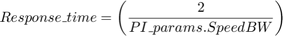
Compare the theoretical Response_time with the actual response time ΔT to validate the speed PI controller gains.
Similarly, you can validate the current PI controller gains by analyzing the step responses of the flux and the d and q current PI controllers.
Troubleshooting
Follow these steps to troubleshoot failed gain-tuning instances.
1. Identify the loop (either d current, q current, flux, or speed) for which the tuning process failed.
The target model tunes the PI controllers in this sequence:
d current controller → q current controller → flux controller → speed controller
Tuning failure of one controller in this sequence results in incorrect gain tuning for the subsequent controllers.
Check the computed gains for the four controllers using the Display blocks available in the host model. A zero Kp or Ki controller gain value indicates that the tuning process failed for the respective controller.
Follow the subsequent steps for the first PI controller in the preceding sequence for which the tuning failed.
2. Select the controller reference and feedback signals for the controller identified in step 1, in the Debug signals section (for example, Iq_Ref & Iq_Feedback for the q current controller) and open the SelectedSignals time scope.
3. Check that the PI Parameters slider switch is in the Autotuner position.
4. Turn the Autotuner slider switch to the Start position to run the tuning process again.
5. Monitor the feedback signal for the controller identified in step 1 (for example, Iq_Feedback) in the SelectedSignals time scope.
Case 1: Follow these steps if the peak value of the controller feedback signal satisfies one of these conditions:
Value is too high (greater than 1)
Value is too low (less than
PI_params.CurrentSineAmpfor the current controllers, less thanPI_params.FluxSineAmpfor the flux controller, or less thanPI_params.SpeedSineAmpfor the speed controller)
Note: The PI_params.CurrentSineAmp, PI_params.FluxSineAmp, and PI_params.SpeedSineAmp variables are defined in the model initialization script.
a. If the controller identified in step 1 is the d or the q current controller, modify the PI_params.CurrentSineAmp variable such that it is less than the peak value of the controller feedback signal.
b. If the controller identified in step 1 is the flux controller, modify the PI_params.FluxSineAmp variable such that it is less than the peak value of the controller feedback signal.
c. If the controller identified in step 1 is the speed controller, modify the PI_params.SpeedSineAmp variable such that it is less than the peak value of the controller feedback signal.
d. Turn the Autotuner slider switch to the Stop position and then to the Start position to run the tuning process again.
Case 2: Follow these steps if the peak value of the controller feedback signal lies in the range:
![$\left[ {PI{\rm{\_}}params.CurrentSineAmp,1} \right]$](../../examples/mcb/win64/TunePIControllersInFWCModeUsingFOCAutotunerBlockExample_eq17210640577894276931.png) (for the current controllers)
(for the current controllers)
![$\left[ {PI{\rm{\_}}params.FluxSineAmp,1} \right]$](../../examples/mcb/win64/TunePIControllersInFWCModeUsingFOCAutotunerBlockExample_eq15927690209159747880.png) (for the flux controller)
(for the flux controller)
![$\left[ {PI{\rm{\_}}params.SpeedSineAmp,1} \right]$](../../examples/mcb/win64/TunePIControllersInFWCModeUsingFOCAutotunerBlockExample_eq02272392176590374417.png) (for the speed controller)
(for the speed controller)
Note: The PI_params.CurrentSineAmp, PI_params.FluxSineAmp, and PI_params.SpeedSineAmp variables are defined in the model initialization script.
a. Update the parameters of the Field Oriented Control Autotuner block (that set the reference bandwidth and phase margin values) available in the FOC Autotuner parameters section of the model initialization script.
b. Turn the Autotuner slider switch to the Stop position and then to the Start position to run the tuning process again.