Automatic Differentiation Background
What Is Automatic Differentiation?
Automatic differentiation (also known as autodiff,
AD, or algorithmic
differentiation) is a widely used tool in optimization. The solve
function uses automatic differentiation by default in problem-based optimization for
general nonlinear objective functions and constraints; see Automatic Differentiation in Optimization Toolbox.
Automatic differentiation is a set of techniques for evaluating derivatives (gradients) numerically. The method uses symbolic rules for differentiation, which are more accurate than finite difference approximations. Unlike a purely symbolic approach, automatic differentiation evaluates expressions numerically early in the computations, rather than carrying out large symbolic computations. In other words, automatic differentiation evaluates derivatives at particular numeric values; it does not construct symbolic expressions for derivatives.
Forward mode automatic differentiation evaluates a numerical derivative by performing elementary derivative operations concurrently with the operations of evaluating the function itself. As detailed in the next section, the software performs these computations on a computational graph.
Reverse mode automatic differentiation uses an extension of the forward mode computational graph to enable the computation of a gradient by a reverse traversal of the graph. As the software runs the code to compute the function and its derivative, it records operations in a data structure called a trace.
As many researchers have noted (for example, Baydin, Pearlmutter, Radul, and
Siskind [1]), for a scalar
function of many variables, reverse mode calculates the gradient more efficiently
than forward mode. Because an objective function is scalar, solve
automatic differentiation uses reverse mode for scalar optimization. However, for
vector-valued functions such as nonlinear least squares and equation solving,
solve uses forward mode for some calculations. See Automatic Differentiation in Optimization Toolbox.
Forward Mode
Consider the problem of evaluating this function and its gradient:
Automatic differentiation works at particular points. In this case, take x1 = 2, x2 = 1/2.
The following computational graph encodes the calculation of the function f(x).
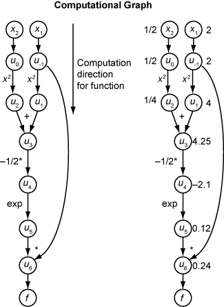
To compute the gradient of f(x) using forward mode, you compute the same graph in the same direction, but modify the computation based on the elementary rules of differentiation. To further simplify the calculation, you fill in the value of the derivative of each subexpression ui as you go. To compute the entire gradient, you must traverse the graph twice, once for the partial derivative with respect to each independent variable. Each subexpression in the chain rule has a numeric value, so the entire expression has the same sort of evaluation graph as the function itself.
The computation is a repeated application of the chain rule. In this example, the derivative of f with respect to x1 expands to this expression:
Let represent the derivative of the expression ui with respect to x1. Using the evaluated values of the ui from the function evaluation, you compute the partial derivative of f with respect to x1 as shown in the following figure. Notice that all the values of the become available as you traverse the graph from top to bottom.
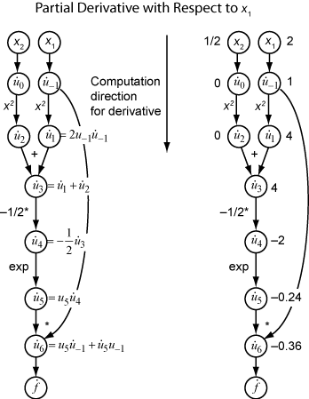
To compute the partial derivative with respect to x2, you traverse a similar computational graph. Therefore, when you compute the gradient of the function, the number of graph traversals is the same as the number of variables. This process can be slow for many applications, when the objective function or nonlinear constraints depend on many variables.
Reverse Mode
Reverse mode uses one forward traversal of a computational graph to set up the trace. Then it computes the entire gradient of the function in one traversal of the graph in the opposite direction. For problems with many variables, this mode is far more efficient.
The theory behind reverse mode is also based on the chain rule, along with associated adjoint variables denoted with an overbar. The adjoint variable for ui is
In terms of the computational graph, each outgoing arrow from a variable contributes to the corresponding adjoint variable by its term in the chain rule. For example, the variable u–1 has outgoing arrows to two variables, u1 and u6. The graph has the associated equation
In this calculation, recalling that and u6 = u5u–1, you obtain
During the forward traversal of the graph, the software calculates the intermediate variables ui. During the reverse traversal, starting from the seed value , the reverse mode computation obtains the adjoint values for all variables. Therefore, reverse mode computes the gradient in just one computation, saving a great deal of time compared to forward mode.
The following figure shows the computation of the gradient in reverse mode for the function
Again, the computation takes x1 = 2, x2 = 1/2. The reverse mode computation relies on the ui values that are obtained during the computation of the function in the original computational graph. In the right portion of the figure, the computed values of the adjoint variables appear next to the adjoint variable names, using the formulas from the left portion of the figure.
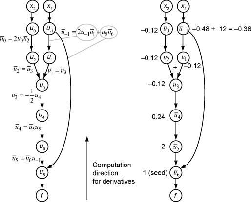
The final gradient values appear as and .
For more details, see Baydin, Pearlmutter, Radul, and Siskind [1] or the Wikipedia article on automatic differentiation [2].
Closed Form
For linear or quadratic objective or constraint functions, gradients are available
explicitly at very low computational cost from the coefficients. In these cases,
solve and prob2struct provide the
gradients explicitly, without going through AD, and applicable solvers always use
the gradients. If you get an output structure, the relevant
objectivederivative or
constraintderivative fields have the value
"closed-form".
Automatic Differentiation in Optimization Toolbox
Automatic differentiation (AD) applies to the solve and
prob2struct
functions under the following conditions:
The objective and constraint functions are supported, as described in Supported Operations for Optimization Variables and Expressions. They do not require use of the
fcn2optimexprfunction.The solver called by
solveisfmincon,fminunc,fsolve, orlsqnonlin.For optimization problems, the
ObjectiveDerivativeandConstraintDerivativename-value arguments forsolveorprob2structare set to"auto"(default),"auto-forward", or"auto-reverse".For equation problems, the
EquationDerivativeoption is set to"auto"(default),"auto-forward", or"auto-reverse".
| When AD Applies | All Constraint Functions Supported | One or More Constraints Not Supported |
|---|---|---|
| Objective Function Supported | AD used for objective and constraints | AD used for objective only |
| Objective Function Not Supported | AD used for constraints only | AD not used |
Note
For linear or quadratic objective or constraint functions, applicable solvers always use explicit function gradients. These gradients are not produced using AD. See Closed Form.
When these conditions are not satisfied, solve estimates gradients by
finite differences, and prob2struct does not create gradients in its
generated function files.
Solvers choose the following type of AD by default:
For a general nonlinear objective function,
fmincondefaults to reverse AD for the objective function.fmincondefaults to reverse AD for the nonlinear constraint function when the number of nonlinear constraints is less than the number of variables. Otherwise,fmincondefaults to forward AD for the nonlinear constraint function.For a general nonlinear objective function,
fminuncdefaults to reverse AD.For a least-squares objective function,
fminconandfminuncdefault to forward AD for the objective function. For the definition of a problem-based least-squares objective function, see Write Objective Function for Problem-Based Least Squares.lsqnonlindefaults to forward AD when the number of elements in the objective vector is greater than or equal to the number of variables. Otherwise,lsqnonlindefaults to reverse AD.fsolvedefaults to forward AD when the number of equations is greater than or equal to the number of variables. Otherwise,fsolvedefaults to reverse AD.
Note
To use automatic derivatives in a problem converted by prob2struct, pass options specifying these derivatives.
options = optimoptions("fmincon",SpecifyObjectiveGradient=true,...
    SpecifyConstraintGradient=true);
problem.options = options;
Currently, AD works only for first derivatives; it does not apply to second or higher
derivatives. So, for example, if you want to use an analytic Hessian to speed your
optimization, you cannot use solve directly, and must instead use the
approach described in Supply Derivatives in Problem-Based Workflow.
References
[1] Baydin, Atilim Gunes, Barak A. Pearlmutter, Alexey Andreyevich Radul, and Jeffrey Mark Siskind. "Automatic Differentiation in Machine Learning: A Survey." The Journal of Machine Learning Research, 18(153), 2018, pp. 1–43. Available at https://arxiv.org/abs/1502.05767.
[2] Automatic differentiation. Wikipedia. Available at https://en.wikipedia.org/wiki/Automatic_differentiation.