Monitor During Parallel Optimizations with parfor
This example shows how to run multiple optimization problems in parallel using parfor, while monitoring solver progress in real time on the client using a DataQueue.
You can use a DataQueue object to send progress data from workers during computations on a parallel pool. If your optimization function supports the OutputFcn option, you can define a custom function that sends progress updates to the client at each iteration with the DataQueue. You can dynamically update plots on the client with this data.
Problem Description
The optimization problem models a system of electrons inside a conducting body. Each electron repels the others, and the goal is to find a configuration that minimizes the total electrostatic potential energy. The optimal configuration spreads the electrons evenly within the constraints of the conducting body. For full problem details, see Constrained Electrostatic Nonlinear Optimization Using Optimization Variables (Optimization Toolbox).
In this example, you solve this problem for varying numbers of electrons in parallel, starting from randomized initial positions on a sphere.
Start a parallel pool of process workers on the local machine.
parpool("Processes");Starting parallel pool (parpool) using the 'Processes' profile ... Connected to parallel pool with 6 workers.
Prepare Plots and Data Queue to Visualize Optimization Progress
Specify the range of electrons and the number of optimizations to run.
electronCounts = 12:20;
numOptims = numel(electronCounts);
Before running the optimizations, set up plots to visualize the evolving electron configurations and the changes in objective function values during the optimization. Use the preparePlots helper function, which is provided at the end of this example, to create figures and plots for each optimization.
[eFig,fFig,hELines,hLines] = preparePlots(electronCounts);
Send the optimization progress updates from the workers to the client by using a DataQueue, and plot the data. Update the plots each time the workers send updates by using afterEach. The parameter data contains information about the electron configuration and objective function values.
queue = parallel.pool.DataQueue;
afterEach(queue,@(data) updatePlots(data{:},hELines,hLines));
Run Optimizations
Visualize the changes in electron configurations during the optimizations.
eFig.Visible = "on";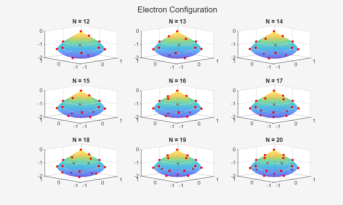
Visualize the changes in the function value during the optimizations.
fFig.Visible = "on";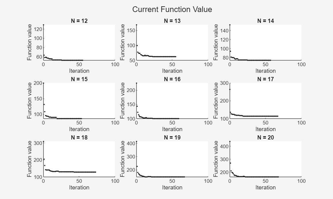
Use a parfor-loop to run multiple optimizations in parallel. For each parfor iteration:
Create the optimization problem using the
createProblemhelper function, which is provided at the end of the example.Generate random initial positions on a sphere.
Define a custom output function,
sendProgress, that sends progress updates to the client. ThesendProgresshelper function is provided at the end of the example. Use an anonymous function to send theDataQueueobject to the workers.Solve the problem and save the results.
parfor idx = 1:numOptims
    N = electronCounts(idx);
    elecProb = createProblem(N)

    % Generate random initial positions on a sphere
    x0 = randn(N,3);
    for c=1:N
        x0(c,:) = x0(c,:)/norm(x0(c,:))/2;
        x0(c,3) = x0(c,3) - 1;
    end
    initPos = struct("x",x0(:,1),"y",x0(:,2),"z",x0(:,3));

    % Prepare custom output function
    default = solvers(elecProb);
    outFcn = @(in,vals,state) sendProgress(in,vals,state,queue,idx);
    opts = optimoptions(default,OutputFcn=outFcn,Display="off");

    [s,f,e,o] = solve(elecProb,initPos,Options=opts);

    sol(idx,:) = s;
    fval(idx) = f;
    eflag(idx) = e;
    output(idx) = o;
end
Analyze Results
After all of the optimizations complete, check the exit flags to verify convergence.
failedIdx = find(eflag~=1);

if isempty(failedIdx)
    disp("All optims converged to an optimal solution.");
else
    fprintf("optims that failed to converge: %s\n",mat2str(failedIdx));
end
All optims converged to an optimal solution.
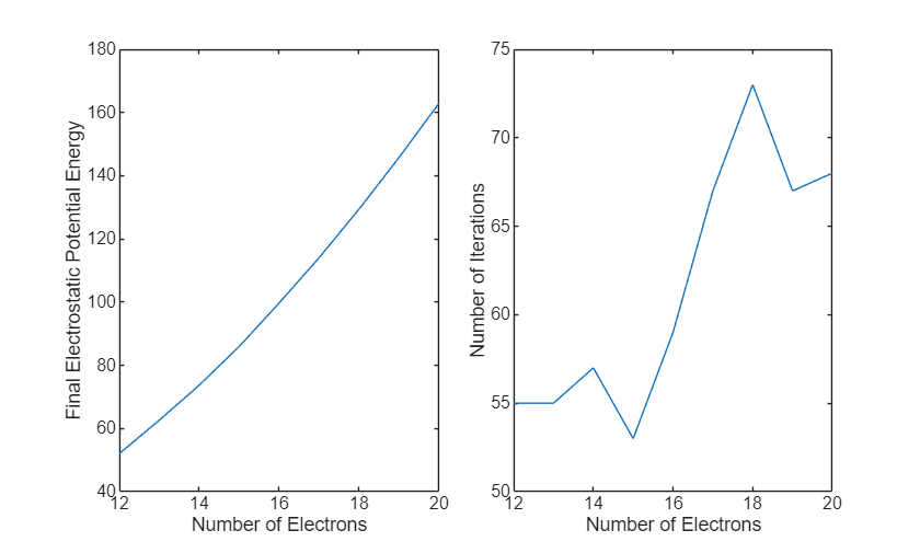
Plot the final potential energy and the number of iterations required for each optimization against the number of electrons. In these results, the final total energy increases with the number of electrons, reflecting the larger number of repelling pairs. The plot of number of iterations versus number of electrons shows how solver convergence changes as the problem size increases, with more iterations indicating slower convergence and fewer iterations indicating faster convergence.
figure;
tiledlayout(1,4);
nexttile([1 2])
plot(electronCounts,fval)
xlabel("Number of Electrons")
ylabel("Final Electrostatic Potential Energy")
nexttile([1 2])
plot(electronCounts,[output(:).iterations])
xlabel("Number of Electrons")
ylabel("Number of Iterations")
Helper Functions
sendProgress Function
The sendProgress function is a custom output function that sends the current solver state and iteration information to the client via a DataQueue object. For more information about the structure of an output function, see Output Function and Plot Function Syntax (Optimization Toolbox).
function stop = sendProgress(in,optimValues,state,queue,plotIdx)
send(queue,{in,optimValues,state,plotIdx});
pause(0.5);
stop = false;
end
updatePlots Function
The updatePlots function updates plots with the progress of an optimization as it runs. The function uses the state input to perform different actions at the start of the optimization, during iterations, and at completion:
On
"init": No action.On
"iter": Update theXData,YData, andZDataproperties of the electron configuration plot to show the current electron positions. Append the current iterate to the animated line to show the trajectory of the solver.On
"done": No action.
For more information about the structure of plot functions, see Output Function and Plot Function Syntax (Optimization Toolbox).
function updatePlots(in,vals,state,plotIdx,hELines,hFLines)
hEl = hELines(plotIdx); % Electron configuration plots
hFl = hFLines(plotIdx); % Function value plots
switch state
    case "init"
        % No action
    case "iter"
        in = reshape(in,[],3);
        hEl.XData = in(:,1);
        hEl.YData = in(:,2);
        hEl.ZData = in(:,3);
        addpoints(hFl,vals.iteration,vals.fval);
        drawnow limitrate nocallbacks;
    case "done"
        % No action
end
end
preparePlots Function
The preparePlots function initializes figures, electron configuration, and animated line plot placeholders for each optimization.
function [eFig,fFig,hELines,hFLines] = preparePlots(electronCounts)
% Prepare plots for each optimization with varying numbers of electrons
numOptims = numel(electronCounts);

hELines = gobjects(1,numOptims);
hFLines = gobjects(1,numOptims);

[X,Y] = meshgrid(-1:.01:1);
Z1 = -abs(X) - abs(Y);
Z2 = -1 - sqrt(1 - X.^2 - Y.^2);
Z2 = real(Z2);

% Mask out regions where Z1 < Z2
W1 = Z1;
W2 = Z2;
W1(Z1 < Z2) = nan;
W2(Z1 < Z2) = nan;

% Geometry figure
eFig = figure(Visible="off");
t1 = tiledlayout(eFig,3,3);
title(t1,"Electron Configuration");

% Function value figure
fFig = figure(Visible="off");
t2 = tiledlayout(fFig,3,3,TileSpacing="tight");
title(t2,"Current Function Value");

for k = 1:numOptims
    % Geometry plot
    ax1 = nexttile(t1,k);
    surf(ax1,X,Y,W1,LineStyle="none",FaceAlpha=0.5);
    hold on
    surf(ax1,X,Y,W2,LineStyle="none",FaceAlpha=0.5);
    view(ax1,-44,18)
    title(ax1,sprintf("N = %d",electronCounts(k)));

    % Placeholder for electron positions
    init = NaN(electronCounts(k),1);
    hELines(k) = plot3(ax1,init,init,init,"r.",MarkerSize=12);
    hold off

    % Function value plot
    ax2 = nexttile(t2,k);
    hFLines(k) = animatedline(ax2,NaN,NaN,...
        Marker=".",LineStyle="none",MaximumNumPoints=200);
    xlabel(ax2,"Iteration");
    ylabel(ax2,"Function value");
    xlim(ax2,[0 100]);
    title(ax2,sprintf("N = %d",electronCounts(k)));
end
end
createProblem Function
The createProblem function defines the optimization variables, constraints, and objective. For full problem details, see Constrained Electrostatic Nonlinear Optimization Using Optimization Variables (Optimization Toolbox).
function elecprob = createProblem(N)
% Define the variables for the problem.
x = optimvar("x",N,"LowerBound",-1,"UpperBound",1);
y = optimvar("y",N,"LowerBound",-1,"UpperBound",1);
z = optimvar("z",N,"LowerBound",-2,"UpperBound",0);
elecprob = optimproblem;

% Define this spherical constraint of a simple polynomial
%  inequality for each electron separately
elecprob.Constraints.spherec = (x.^2 + y.^2 + (z+1).^2) <= 1;

% Write the absolute value constraint as four linear inequalities.
% Each constraint command returns a vector of N constraints.
elecprob.Constraints.plane1 = z <= -x-y;
elecprob.Constraints.plane2 = z <= -x+y;
elecprob.Constraints.plane3 = z <= x-y;
elecprob.Constraints.plane4 = z <= x+y;

% The objective function is the potential energy of the system,
% which is a sum over each electron pair of the inverse
% of their distances:
% energy = SUM[1/||electron(i) - electron(j)||]
% Define the objective function as an optimization expression.
energy = optimexpr(1);
for ii = 1:(N-1)
    jj = (ii+1):N;
    tE = (x(ii)-x(jj)).^2 + (y(ii)-y(jj)).^2 + (z(ii)-z(jj)).^2;
    energy = energy + sum(tE.^(-1/2));
end
elecprob.Objective = energy;
end