Modal and Frequency Response Analysis for Single Part of Kinova Gen3 Robotic Arm
This example shows how to analyze the shoulder link of a Kinova® Gen3 Ultra lightweight robotic arm for possible deformation under pressure.
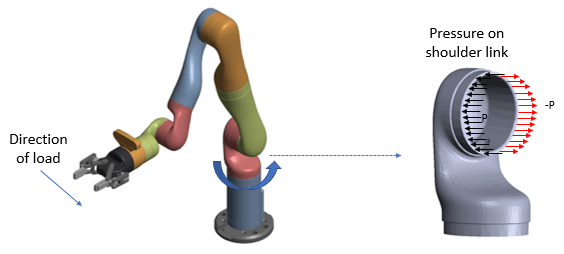
Robotic arms perform precise manipulations in a wide variety of applications from factory automation to medical surgery. Typically, robotic arms consist of several links connected in a serial chain, with a base attached to a tabletop or the ground and an end-effector attached at the tip. These links must be structurally strong to avoid any vibrations when the rotors are moving with a load on them.
Loads at the tips of a robotic arm cause pressure on the joints of each link. The direction of pressure depends on the direction of the load.
This example computes deformations of the shoulder link under applied pressure by performing a modal analysis and frequency response analysis simulation.
Modal Analysis
Assuming that one end of the robotic arm is fixed, find the natural frequencies and mode shapes.
Create an femodel object for modal structural analysis and include the geometry of the shoulder part of the robotic arm.
model = femodel(AnalysisType="StructuralModal", ...
                Geometry="Gen3Shoulder.stl");
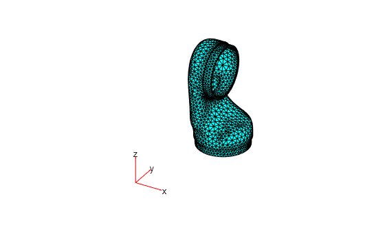
Generate and plot a mesh.
model = generateMesh(model);
pdemesh(model)
Specify Young's modulus, Poisson's ratio, and the mass density of the material in consistent units. Typically, the material used for the link is carbon fiber reinforced plastic. Assume that the material is homogeneous.
E = 1.5e11;
nu = 0.3;
rho = 2000;
model.MaterialProperties = ...
    materialProperties(YoungsModulus=E, ...
                       PoissonsRatio=nu, ...
                       MassDensity=rho);
Identify faces for applying boundary constraints and loads by plotting the geometry with the face labels.
pdegplot(model.Geometry,FaceLabels="on")
view([-1 2])
title("Shoulder Link Geometry with Face Labels")
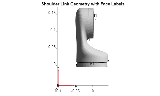
The shoulder link is fixed on one end (face 3) and connected to a moving link on the other end (face 4). Apply the fixed boundary condition on face 3.
model.FaceBC(3) = faceBC(Constraint="fixed");Solve the model for a chosen frequency range. Specify the lower frequency limit below zero so that all modes with frequencies near zero, if any, appear in the solution.
RF = solve(model,FrequencyRange=[-1,10000]*2*pi);
By default, the solver returns circular frequencies.
modeID = 1:numel(RF.NaturalFrequencies);
Express the resulting frequencies in Hz by dividing them by . Display the frequencies in a table.
tmodalResults = table(modeID.',RF.NaturalFrequencies/2/pi);
tmodalResults.Properties.VariableNames = {'Mode','Frequency'};
disp(tmodalResults);
Mode Frequency
____ _________
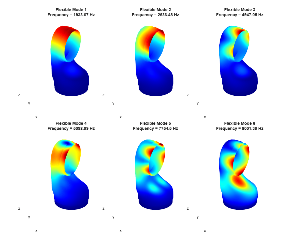
1 1933.7
2 2636.5
3 4947.1
4 5099
5 7754.5
6 8001.4
7 9127.3
The best way to visualize the mode shapes is to animate the harmonic motion at their respective frequencies. The animateSixLinkModes function animates the first six modes. The resulting plot shows the areas of dominant deformation under load.
frames = animateSixLinkModes(RF);
To play the animation, use this command:
movie(figure("units","normalized","outerposition",[0 0 1 1]),frames,5,30)
Frequency Response Analysis
Simulate the dynamics of the shoulder under pressure loading on a face, assuming that the attached link applies an equal and opposite amount of pressure on the halves of the face. Analyze the frequency response and deformation of a point in the face.

Change the analysis type to the frequency response analysis.
model.AnalysisType = "StructuralFrequency";Estimate the pressure that the moving link applies on face 4 when the arm carries a load. This figure shows two halves of face 4 divided at the center along the y-coordinate.
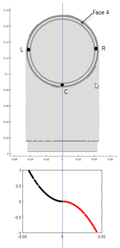
Use the pressFcnFR function to apply the boundary load on face 4. This function applies a push and a twist pressure signal. The push pressure component is uniform. The twist pressure component applies positive pressure on the left side and negative pressure on the right side of the face. For the definition of the pressFcnFR function, see Pressure Function. This function does not have an explicit dependency on frequency. Therefore, in the frequency domain, this pressure load acts across all frequencies of the solution.
model.FaceLoad(4) = ...
    faceLoad(Pressure=@(region,state)pressFcnFR(region,state));
Define the frequency list for the solution as 0 to 3500 Hz with 200 steps.
flist = linspace(0,3500,200)*2*pi;
Solve the model using the modal frequency response solver by specifying the modal results object RF as one of the inputs.
R = solve(model,flist,ModalResults=RF);
Plot the frequency response at a point on the loaded face. A point on face 4 located at maximum negative pressure loading is (0.003; 0.0436; 0.1307). Interpolate the displacement to this point and plot the result.
queryPoint  = [0.003; 0.0436; 0.1307];
queryPointDisp = interpolateDisplacement(R,queryPoint);

figure
plot(R.SolutionFrequencies/2/pi,abs(queryPointDisp.uy))
title("Transverse Displacement at a Point on a Loaded Face")
xlabel("Frequency (Hz)")
ylabel("Y-Displacement")
xlim([0.0000 3500])
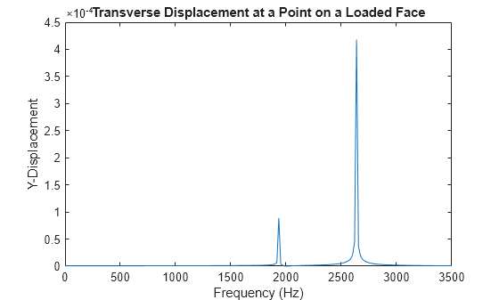
The peak of the response occurs near 2700 Hz, which is close to the second mode of vibration. A smaller response also occurs at the first mode close to 1950 Hz.
Find the peak response frequency index by using the max function with two output arguments. The second output argument provides the index of the peak frequency.
[M,I] = max(abs(queryPointDisp.uy))
M =
4.1798e-04
I =
151
Find the peak response frequency value in Hz.
R.SolutionFrequencies(152)/2/pi
ans =
2.6558e+03
Plot the deformation at the peak response frequency. The applied load is such that it predominantly excites the opening mode and the bending mode of the shoulder.
RD = struct();
RD.ux = R.Displacement.ux(:,I);
RD.uy = R.Displacement.uy(:,I);
RD.uz = R.Displacement.uz(:,I);

nexttile
pdeplot3D(R.Mesh,ColorMapData=R.Displacement.ux(:,I), ...
                 Deformation=RD,DeformationScaleFactor=1);
title("x-Displacement")

nexttile
pdeplot3D(R.Mesh,ColorMapData=R.Displacement.uy(:,I), ...
                 Deformation=RD,DeformationScaleFactor=1);
title("y-Displacement")

nexttile
pdeplot3D(R.Mesh,ColorMapData=R.Displacement.uz(:,I), ...
                 Deformation=RD,DeformationScaleFactor=1);
title("z-Displacement")
nexttile
%subplot(2,2,4)
pdeplot3D(R.Mesh,ColorMapData=R.Displacement.Magnitude(:,I), ...
                 Deformation=RD,DeformationScaleFactor=1);
title("Magnitude")

Clear figure for future plots.
clf
You also can plot the same results by using the Visualize PDE Results Live Editor task. First, create a new live script by clicking the New Live Script button in the File section on the Home tab.

On the Live Editor tab, select Task > Visualize PDE Results. This action inserts the task into your script.

Plot the components and the magnitude of the displacement at the peak response frequency. To plot the x-displacement, follow these steps. To plot the y- and z-displacements and the magnitude, follow the same steps, but set Component to Y, Z, and Magnitude, respectively.
In the Select results section of the task, select
Rfrom the drop-down menu.In the Specify data parameters section of the task, set Type to Displacement, Component to X, and Frequency to 2655.7789 Hz.
In the Specify visualization parameters section of the task, clear the Deformation check box.
% Data to visualize
meshData = R.Mesh;
nodalData = R.Displacement.ux(:,152);
deformationData = [R.Displacement.ux(:,152) ...
    R.Displacement.uy(:,152) ...
    R.Displacement.uz(:,152)];
phaseData = cospi(0) + 1i*sinpi(0);

% Create PDE result visualization
resultViz = pdeviz(meshData,nodalData*phaseData, ...
    "DeformationData",deformationData*phaseData, ...
    "DeformationScaleFactor",0, ...
    "ColorLimits",[-7.414e-05 7.414e-05]);

% Clear temporary variables
clearvars meshData nodalData deformationData phaseData
Pressure Function
Define a pressure function, pressFcnFR, to calculate a push and a twist pressure signal. The push pressure component is uniform. The twist pressure component applies positive pressure on the left side and negative pressure on the right side of the face. The value of the twist pressure loading increases in a parabolic distribution from the minimum at point C to the positive peak at L and to the negative peak at R. The twist pressure factor for the parabolic distribution obtained in pressFcnFR is multiplied with a sinusoidal function with a magnitude of 0.1 MPa. The uniform push pressure value is 10 kPa.
function p = pressFcnFR(region,~)

meanY = mean(region.y);
absMaxY = max(abs(region.y));
scaleFactor = zeros(size(region.y));

% Find IDs of the points on the left
% and right halves of the face
% using y-coordinate values.
leftHalfIdx = region.y <= meanY;
rightHalfIdx = region.y >= meanY;

% Define a parabolic scale factor
% for each half of the face.
scaleFactor(leftHalfIdx) = ...
    ((region.y(leftHalfIdx) - meanY)/absMaxY).^2;
scaleFactor(rightHalfIdx) = ...
   -((region.y(rightHalfIdx) - meanY)/absMaxY).^2;

p = 10E3 + 0.1E6*scaleFactor;

end