plotResponse
System object: phased.RangeResponse
Namespace: phased
Plot range response
Syntax
Description
plotResponse(
plots
the range response with additional options specified by one or more response
,___,Name,Value
)Name,Value
pair
arguments.
Input Arguments
response
— Range response
phased.RangeResponse
System object™
Range response, specified as a phased.RangeResponse
System object.
Example: phased.RangeResponse
x
— Input radar data
complex-valued K-element column vector | complex-valued K-by-N
matrix
Input radar data, specified as a complex-valued K-by-1 column vector, or K-by-N matrix.
K is the number of fast-time or range samples. Each K-element fast-time dimension is processed independently.
N is the number of independent spatial channels such as sensors or directions.
For FMCW waveforms with a triangle sweep, the sweeps alternate between
positive and negative slopes. However, phased.RangeResponse
is designed to process consecutive
sweeps of the same slope. To apply phased.RangeResponse
for a triangle-sweep system, use one of
the following approaches:
Specify a positive
SweepSlope
property value, withx
corresponding to upsweeps only. After obtaining the Doppler or speed values, divide them by 2.Specify a negative
SweepSlope
property value, withx
corresponding to downsweeps only. After obtaining the Doppler or speed values, divide them by 2.
The size of the first dimension of the input matrix can vary to simulate a changing signal length. A size change can occur, for example, in the case of a pulse waveform with variable pulse repetition frequency.
Data Types: single
| double
Complex Number Support: Yes
xref
— Reference signal used for dechirping
complex-valued K-by-1 column vector
Reference signal used for dechirping, specified as a complex-valued K-by-1
column vector. The value of K must equal the length
of the first dimension of x
.
Dependencies
To enable this input argument, set the value of RangeMethod
to 'FFT'
and DechirpInput
to true
.
Data Types: single
| double
Complex Number Support: Yes
coeff
— Matched filter coefficients
complex-valued P-by-1 column vector
Matched filter coefficients, specified as a complex-valued P-by-1 column vector. P must be less than or equal to K, the length of the fast-time dimension.
Dependencies
To enable this input argument, set RangeMethod
property
to 'Matched filter'
.
Data Types: single
| double
Complex Number Support: Yes
Name-Value Arguments
Specify optional pairs of arguments as
Name1=Value1,...,NameN=ValueN
, where Name
is
the argument name and Value
is the corresponding value.
Name-value arguments must appear after other arguments, but the order of the
pairs does not matter.
Before R2021a, use commas to separate each name and value, and enclose
Name
in quotes.
Unit
— Vertical axes units
'db'
(default) | 'mag'
| 'pow'
Units for vertical axis of plot, specified as 'db'
, 'mag'
,
or 'pow'
.
Example: 'pow'
Data Types: char
Examples
Plot Range Response of Three Targets
Plot the radar range response of three targets using the plotResponse
method of the phased.RangeResponse
System object™. The transmitter and receiver are collocated isotropic antenna elements forming a monostatic radar system. The transmitted signal is a linear FM waveform with a pulse repetition interval of 7.0 μs and a duty cycle of 2%. The operating frequency is 77 GHz and the sample rate is 150 MHz.
fs = 150e6;fs = 150e6;
c = physconst('LightSpeed');
fc = 77e9;
pri = 7e-6;
prf = 1/pri;
Set up the scenario parameters. The radar transmitter and receiver are stationary and located at the origin. The targets are 500, 530, and 750 meters from the radars on the x-axis. The targets move along the x-axis at speeds of −60, 20, and 40 m/s. All three targets have a nonfluctuating RCS of 10 dB.
Create the target and radar platforms.
Numtgts = 3; tgtpos = zeros(Numtgts); tgtpos(1,:) = [500 530 750]; tgtvel = zeros(3,Numtgts); tgtvel(1,:) = [-60 20 40]; tgtrcs = db2pow(10)*[1 1 1]; tgtmotion = phased.Platform(tgtpos,tgtvel); target = phased.RadarTarget('PropagationSpeed',c,'OperatingFrequency',fc, ... 'MeanRCS',tgtrcs); radarpos = [0;0;0]; radarvel = [0;0;0]; radarmotion = phased.Platform(radarpos,radarvel);
Create the transmitter and receiver antennas.
txantenna = phased.IsotropicAntennaElement; rxantenna = clone(txantenna);
Set up the transmitter-end signal processing. Construct an upsweep linear FM signal with a bandwidth of half the sample rate. Find the rms bandwidth and rms range resolution.
bw = fs/2; waveform = phased.LinearFMWaveform('SampleRate',fs,... 'PRF',prf,'OutputFormat','Pulses','NumPulses',1,'SweepBandwidth',fs/2,... 'DurationSpecification','Duty cycle','DutyCycle',.02); sig = waveform(); Nr = length(sig); bwrms = bandwidth(waveform)/sqrt(12); rngrms = c/bwrms;
Set up the transmitter and radiator System object properties. The peak output power is 10 W and the transmitter gain is 36 dB.
peakpower = 10; txgain = 36.0; transmitter = phased.Transmitter(... 'PeakPower',peakpower,... 'Gain',txgain,... 'InUseOutputPort',true); radiator = phased.Radiator(... 'Sensor',txantenna,... 'PropagationSpeed',c,... 'OperatingFrequency',fc);
Create a free-space propagation channel in two-way propagation mode.
channel = phased.FreeSpace(... 'SampleRate',fs,... 'PropagationSpeed',c,... 'OperatingFrequency',fc,... 'TwoWayPropagation',true);
Set up the receiver-end processing. The receiver gain is 42 dB and noise figure is 10.
collector = phased.Collector(... 'Sensor',rxantenna,... 'PropagationSpeed',c,... 'OperatingFrequency',fc); rxgain = 42.0; noisefig = 10; receiver = phased.ReceiverPreamp(... 'SampleRate',fs,... 'Gain',rxgain,... 'NoiseFigure',noisefig);
Loop over 128 pulses to build a data cube. For each step of the loop, move the target and propagate the signal. Then put the received signal into the data cube. The data cube contains the received signal per pulse. Ordinarily, a data cube has three dimensions. The last dimension corresponds to antennas or beams. Because only one sensor is used in this example, the cube has only two dimensions.
The processing steps are:
Move the radar and targets.
Transmit a waveform.
Propagate the waveform signal to the target.
Reflect the signal from the target.
Propagate the waveform back to the radar. Two-way propagation mode allows the return propagation to be combined with the outbound propagation.
Receive the signal at the radar.
Load the signal into the data cube.
Np = 128; cube = zeros(Nr,Np); for n = 1:Np [sensorpos,sensorvel] = radarmotion(pri); [tgtpos,tgtvel] = tgtmotion(pri); [tgtrng,tgtang] = rangeangle(tgtpos,sensorpos); sig = waveform(); [txsig,txstatus] = transmitter(sig); txsig = radiator(txsig,tgtang); txsig = channel(txsig,sensorpos,tgtpos,sensorvel,tgtvel); tgtsig = target(txsig); rxcol = collector(tgtsig,tgtang); rxsig = receiver(rxcol); cube(:,n) = rxsig; end
Create a phased.RangeResponse
System object in matched filter mode. Then, call the plotResponse
method to show the first 20 pulses.
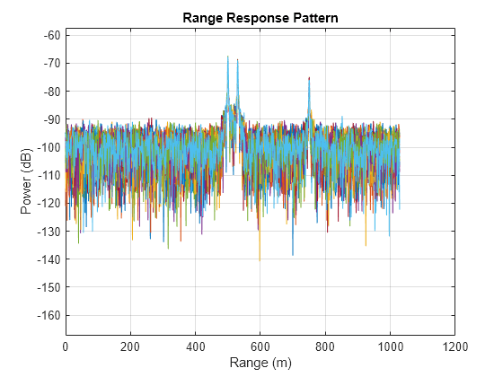
matchcoeff = getMatchedFilter(waveform); rangeresp = phased.RangeResponse('SampleRate',fs,'PropagationSpeed',c); plotResponse(rangeresp,cube(:,1:20),matchcoeff);
Version History
Introduced in R2017a
MATLAB Command
You clicked a link that corresponds to this MATLAB command:
Run the command by entering it in the MATLAB Command Window. Web browsers do not support MATLAB commands.
Select a Web Site
Choose a web site to get translated content where available and see local events and offers. Based on your location, we recommend that you select: .
You can also select a web site from the following list:
How to Get Best Site Performance
Select the China site (in Chinese or English) for best site performance. Other MathWorks country sites are not optimized for visits from your location.
Americas
- América Latina (Español)
- Canada (English)
- United States (English)
Europe
- Belgium (English)
- Denmark (English)
- Deutschland (Deutsch)
- España (Español)
- Finland (English)
- France (Français)
- Ireland (English)
- Italia (Italiano)
- Luxembourg (English)
- Netherlands (English)
- Norway (English)
- Österreich (Deutsch)
- Portugal (English)
- Sweden (English)
- Switzerland
- United Kingdom (English)