Main Content

phased.RangeResponse

Range response

Description

The phased.RangeResponse System object™ performs range filtering on fast-time (range) data, using either a matched filter or an FFT-based algorithm. The output is typically used as input to a detector. Matched filtering improves the SNR of pulsed waveforms. For continuous FM signals, FFT processing extracts the beat frequency of FMCW waveforms. Beat frequency is directly related to range.

The input to the range response object is a radar data cube. The organization of the data cube follows the Phased Array System Toolbox™ convention.

  • The first dimension of the cube represents the fast-time samples or ranges of the received signals.

  • The second dimension represents multiple spatial channels, such as different sensors or beams.

  • The third dimension, slow-time, represents pulses.

Range filtering operates along the fast-time dimension of the cube. Processing along the other dimensions is not performed. If the data contains only one channel or pulse, the data cube can contain fewer than three dimensions. Because this object performs no Doppler processing, you can use the object to process noncoherent radar pulses.

The output of the range response object is also a data cube with the same number of dimensions as the input. Its first dimension contains range-processed data but its length can differ from the first dimension of the input data cube.

To compute the range response:

  1. Create the phased.RangeResponse object and set its properties.

  2. Call the object with arguments, as if it were a function.

To learn more about how System objects work, see What Are System Objects?

Creation

Description

response = phased.RangeResponse creates a range response System object, response.

response = phased.RangeResponse(Name=Value) creates a System object, response, with each specified property Name set to the specified Value. You can specify additional name and value pair arguments in any order as (Name1=Value1,...,NameN=ValueN).

Properties

expand all

Unless otherwise indicated, properties are nontunable, which means you cannot change their values after calling the object. Objects lock when you call them, and the release function unlocks them.

If a property is tunable, you can change its value at any time.

For more information on changing property values, see System Design in MATLAB Using System Objects.

Range response, specified as a phased.RangeResponse System object.

Example: phased.RangeResponse

Measurement mode, specified as "Monostatic" or "Bistatic". When set to "Monostatic", the range measurement is the monostatic range. When set to "Bistatic", the range measurement is the bistatic range.

Example: Mode = "Bistatic"

Data Types: char | string

Range processing method, specified as "Matched filter" or "FFT".

  • "Matched filter" — The object match-filters the incoming signal. This approach is commonly used for pulsed signals, where the matched filter is the time-reverse conjugate of the transmitted signal.

  • "FFT" — The object applies an FFT to the input signal. This approach is commonly used for chirped signals such as FMCW and linear FM pulsed signals.

Example: "Matched filter"

Data Types: char | string

Signal propagation speed, specified as a real-valued positive scalar. Units are in meters per second. The default propagation speed is the value returned by physconst("LightSpeed").

Example: 3e8

Data Types: single | double

Signal sample rate, specified as a positive real-valued scalar. Units are in hertz.

Example: 1e6

Data Types: single | double

Linear FM sweep slope, specified as a scalar. The fast-time dimension of the signal input argument to the object must correspond to sweeps having this slope.

Example: 1.5e9

Dependencies

To enable this property, set the RangeMethod property to "FFT".

Data Types: single | double

Option to enable dechirping of input signals, specified as false or true. Set this property to false to indicate that the input signal is already dechirped and no dechirp operation is necessary. Set this property to true when the input signal requires dechirping.

Dependencies

To enable this property, set the RangeMethod property to "FFT".

Data Types: logical

Decimation factor for dechirped signals, specified as a positive integer. The decimation algorithm uses a 30th-order FIR filter generated by fir1(30,1/D), where D is the decimation factor. The default value of 1 implies no decimation.

When processing FMCW signals, decimating the dechirped signal is useful for reducing the load on A/D converters.

Dependencies

To enable this property, set the RangeMethod property to "FFT" and the DechirpInput property to true.

Data Types: single | double

Source of the FFT length used for the range processing of dechirped signals, specified as "Auto" or "Property".

  • "Auto" — The FFT length equals the length of the fast-time dimension of the input data cube.

  • "Property" — Specify the FFT length by using the RangeFFTLength property.

Dependencies

To enable this property, set the RangeMethod property to "FFT".

Data Types: char | string

FFT length used for range processing, specified as a positive integer.

Dependencies

To enable this property, set the RangeMethod property to "FFT" and the RangeFFTLengthSource property to "Property"

Data Types: single | double

FFT weighting window for range processing, specified as "None", "Hamming", "Chebyshev", "Hann", "Kaiser", "Taylor", or "Custom".

If you set this property to "Taylor", the generated Taylor window has four nearly constant sidelobes next to the mainlobe.

Dependencies

To enable this property, set the RangeMethod property to "FFT".

Data Types: char | string

Sidelobe attenuation for range processing, specified as a positive scalar. Attenuation applies to Kaiser, Chebyshev, or Taylor windows. Units are in dB.

Dependencies

To enable this property, set the RangeMethod property to "FFT" and the RangeWindow property to "Kaiser", "Chebyshev", or "Taylor".

Data Types: single | double

Custom window for range processing, specified as a function handle or a cell array containing a function handle as its first entry. If you do not specify a window length, the object computes the window length and passes that into the function. If you specify a cell array, the remaining cells of the array can contain arguments to the function. If you use only the function handle without passing in arguments, all arguments take their default values.

If you write your own window function, the first argument must be the length of the window.

Note

Instead of using a cell array, you can pass in all arguments by constructing a handle to an anonymous function. For example, you can set the value of CustomRangeWindow to @(n)taylorwin(n,nbar,sll), where you have previously set the values of nbar and sll.

Example: {@taylor,5,-35}

Dependencies

To enable this property, set the RangeMethod property to "FFT" and the RangeWindow property to "Custom".

Data Types: function_handle | cell

Set reference range at center of range grid, specified as true or false. Setting this property to true enables you to set the reference range at the center of the range grid. Setting this property to false sets the reference range to the beginning of the range grid.

Dependencies

To enable this property, set the RangeMethod to "FFT".

Data Types: logical

Reference range of the range grid, specified as a nonnegative scalar.

  • If you set the RangeMethod property to "Matched filter", the reference range is set to the start of the range grid.

  • If you set the RangeMethod property to "FFT", the reference range is determined by the ReferenceRangeCentered property.

    • When you set the ReferenceRangeCentered property to true, the reference range is set to the center of the range grid.

    • When you set the ReferenceRangeCentered property to false, the reference range is set to the start of the range grid.

    Units are in meters.

This property is tunable.

Example: 1000.0

Data Types: single | double

The source of the maximum number of samples the input signal, specified as "Auto" or "Property". When you set this property to "Auto", the object automatically allocates enough memory to buffer the first input signal. When you set this property to "Property", you specify the maximum number of samples in the input signal using the MaximumNumInputSamples property. Any input signal longer than that value is truncated.

Example: "Property"

Dependencies

To use this object with variable-size input signals in a MATLAB® Function Block in Simulink®, set the MaximumNumInputSamplesSource property to "Property" and set a value of the MaximumNumInputSamples property.

Data Types: char | string

Maximum number of samples in the input signal, specified as a positive integer. Any input signal longer than this value is truncated. The input signal is the first argument to the step method. The number of samples is the number of rows in the input.

Example: 2048

Dependencies

To enable this property, set the RangeMethod property to "Matched filter" and set the MaximumNumInputSamplesSource property to "Property".

Data Types: single | double

Number of initial samples in the input signal that should be accounted for due to signal latency, specified as a non-negative.integer. These samples represent the time delay before the relevant signal data begins. Set this property to a non-negative integer value to ensure that the range response calculation starts at the correct point in the signal. Units are in samples.

Example: 6

Data Types: single | double

Usage

Description

[resp,rnggrid] = response(x) computes the range response, resp, for the input signal, x, and the range values, rnggrid, corresponding to the response. This syntax applies when you set RangeMethod to "FFT" and DechirpInput to false. This syntax assumes that the input signal has already been dechirped. This syntax is most commonly used with FMCW signals.

[resp,rnggrid] = response(x,xref) computes the range response of the input signal, x using the reference signal, xref. This syntax applies when you set RangeMethod to "FFT" and DechirpInput to true. Often, the reference signal is the transmitted signal. This syntax assumes that the input signal has not been dechirped. This syntax is most commonly used with FMCW signals.

[resp,rnggrid] = response(x,coeff) computes the range response of x using the matched filter coeff. This syntax applies when you set RangeMethod to "Matched filter". This syntax is most commonly used with pulsed signals.

example

Note

The object performs an initialization the first time the object is executed. This initialization locks nontunable properties and input specifications, such as dimensions, complexity, and data type of the input data. If you change a nontunable property or an input specification, the System object issues an error. To change nontunable properties or inputs, you must first call the release method to unlock the object.

Input Arguments

expand all

Input radar data cube, specified as a complex-valued K-by-1 column vector, a K-by-L matrix, or K-by-N-by-L array.

  • K is the number of fast-time or range samples.

  • N is the number of independent spatial channels such as sensors or directions.

  • L is the slow-time dimension that corresponds to the number of pulses or sweeps in the input signal.

See Radar Data Cube.

Each K-element fast-time dimension is processed independently.

For FMCW waveforms with a triangle sweep, the sweeps alternate between positive and negative slopes. However, phased.RangeResponse is designed to process consecutive sweeps of the same slope. To apply phased.RangeResponse for a triangle-sweep system, use one of the following approaches:

  • Specify a positive SweepSlope property value, with x corresponding to upsweeps only. After obtaining the Doppler or speed values, divide them by 2.

  • Specify a negative SweepSlope property value, with x corresponding to downsweeps only. After obtaining the Doppler or speed values, divide them by 2.

The size of the first dimension of the input matrix can vary to simulate a changing signal length. A size change can occur, for example, in the case of a pulse waveform with variable pulse repetition frequency.

Data Types: single | double
Complex Number Support: Yes

Reference signal used for dechirping, specified as a complex-valued K-by-1 column vector. The number of rows must equal the length of the fast-time dimension of x.

Dependencies

To enable this input argument, set the value of RangeMethod to 'FFT' and DechirpInput to true.

Data Types: single | double
Complex Number Support: Yes

Matched filter coefficients, specified as a complex-valued P-by-1 column vector. P must be less than or equal to K. K is the number of fast-time or range sample.

Dependencies

To enable this input argument, set the value of RangeMethod to 'Matched filter'.

Data Types: double
Complex Number Support: Yes

Output Arguments

expand all

Range response data cube, returned as one of the following:

  • Complex-valued M-element column vector

  • Complex-valued M-by-L matrix

  • Complex-valued M-by-N by-L array

The value of M depends on the type of processing

RangeMethod PropertyDechirpInput PropertyValue of M
"FFT"false

If you set the RangeFFTLength property to "Auto", M = K, the length of the fast-time dimension of x. Otherwise, M equals the value of the RangeFFTLength property.

trueM equals the quotient of the number of rows, K, of the input signal by the value of the decimation factor, D, specified in DecimationFactor.
"Matched filter"n/aM = K, the length of the fast-time dimension of x.

Data Types: single | double
Complex Number Support: Yes

Range values along range dimension, returned as a real-valued M-by-1 column vector. rnggrid defines the ranges corresponding to the fast-time dimension of the resp output data cube. M is the length of the fast-time dimension of resp. Range values are monotonically increasing and equally spaced. Units are in meters.

Example: [0,0.1,0.2,0.3]

Data Types: single | double

Object Functions

To use an object function, specify the System object as the first input argument. For example, to release system resources of a System object named obj, use this syntax:

release(obj)

expand all

plotResponsePlot range response
stepRun System object algorithm
releaseRelease resources and allow changes to System object property values and input characteristics
resetReset internal states of System object

Examples

collapse all

Compute the radar range response of three targets by using the phased.RangeResponse System object™. The transmitter and receiver are collocated isotropic antenna elements forming a monostatic radar system. The transmitted signal is a linear FM waveform with a pulse repetition interval of 7.0 μs and a duty cycle of 2%. The operating frequency is 77 GHz and the sample rate is 150 MHz.

fs = 150e6;
c = physconst("LightSpeed");
fc = 77e9;
pri = 7e-6;
prf = 1/pri;

Set up the scenario parameters. The radar transmitter and receiver are stationary and located at the origin. The targets are 500, 530, and 750 meters from the radars on the x-axis. The targets move along the x-axis at speeds of −60, 20, and 40 m/s. All three targets have a nonfluctuating radar cross-section (RCS) of 10 dB.

Create the target and radar platforms.

Numtgts = 3;
tgtpos = zeros(Numtgts);
tgtpos(1,:) = [500 530 750];
tgtvel = zeros(3,Numtgts);
tgtvel(1,:) = [-60 20 40];
tgtrcs = db2pow(10)*[1 1 1];
tgtmotion = phased.Platform(tgtpos,tgtvel);
target = phased.RadarTarget(PropagationSpeed=c,OperatingFrequency=fc, ...
    MeanRCS=tgtrcs);
radarpos = [0;0;0];
radarvel = [0;0;0];
radarmotion = phased.Platform(radarpos,radarvel);

Create the transmitter and receiver antennas.

txantenna = phased.IsotropicAntennaElement;
rxantenna = clone(txantenna);

Set up the transmitter-end signal processing. Create an upsweep linear FM signal with a bandwidth of half the sample rate. Find the length of the pri in samples and then estimate the rms bandwidth and range resolution.

bw = fs/2;
waveform = phased.LinearFMWaveform(SampleRate=fs, ...
    PRF=prf,OutputFormat="Pulses",NumPulses=1,SweepBandwidth=fs/2, ...
    DurationSpecification="Duty cycle",DutyCycle=0.02);
sig = waveform();
Nr = length(sig);
bwrms = bandwidth(waveform)/sqrt(12);
rngrms = c/bwrms;

Set up the transmitter and radiator System object properties. The peak output power is 10 W and the transmitter gain is 36 dB.

peakpower = 10;
txgain = 36.0;
transmitter = phased.Transmitter( ...
    PeakPower=peakpower, ...
    Gain=txgain, ...
    InUseOutputPort=true);
radiator = phased.Radiator( ...
    Sensor=txantenna, ...
    PropagationSpeed=c, ...
    OperatingFrequency=fc);

Create a free-space propagation channel in two-way propagation mode.

channel = phased.FreeSpace( ...
    SampleRate=fs, ...    
    PropagationSpeed=c, ...
    OperatingFrequency=fc, ...
    TwoWayPropagation=true);

Set up the receiver-end processing. The receiver gain is 42 dB and noise figure is 10.

collector = phased.Collector( ...
    Sensor=rxantenna, ...
    PropagationSpeed=c, ...
    OperatingFrequency=fc);
rxgain = 42.0;
noisefig = 10;
receiver = phased.ReceiverPreamp( ...
    SampleRate=fs, ...
    Gain=rxgain, ...
    NoiseFigure=noisefig);

Loop over 128 pulses to build a data cube. For each step of the loop, move the target and propagate the signal. Then put the received signal into the data cube. The data cube contains the received signal per pulse. Ordinarily, a data cube has three dimensions, where last dimension corresponds to antennas or beams. Because only one sensor is used in this example, the cube has only two dimensions.

The processing steps are:

  1. Move the radar and targets.

  2. Transmit a waveform.

  3. Propagate the waveform signal to the target.

  4. Reflect the signal from the target.

  5. Propagate the waveform back to the radar. Two-way propagation mode enables you to combine the returned propagation with the outbound propagation.

  6. Receive the signal at the radar.

  7. Load the signal into the data cube.

Np = 128;
cube = zeros(Nr,Np);
for n = 1:Np
    [sensorpos,sensorvel] = radarmotion(pri);
    [tgtpos,tgtvel] = tgtmotion(pri);
    [tgtrng,tgtang] = rangeangle(tgtpos,sensorpos);
    sig = waveform();
    [txsig,txstatus] = transmitter(sig);
    txsig = radiator(txsig,tgtang);
    txsig = channel(txsig,sensorpos,tgtpos,sensorvel,tgtvel);    
    tgtsig = target(txsig);   
    rxcol = collector(tgtsig,tgtang);
    rxsig = receiver(rxcol);
    cube(:,n) = rxsig;
end

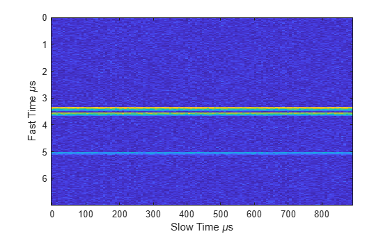
Display the image of the data cube containing signals per pulse.

imagesc([0:(Np-1)]*pri*1e6,[0:(Nr-1)]/fs*1e6,abs(cube))
xlabel('Slow Time {\mu}s')
ylabel('Fast Time {\mu}s')

Figure contains an axes object. The axes object with xlabel Slow Time mu s, ylabel Fast Time mu s contains an object of type image.

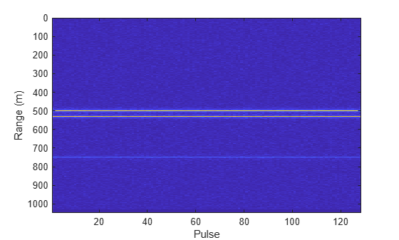
Create a phased.RangeResponse System object in matched filter mode. Then, display the range response image for the 128 pulses. The image shows range vertically and pulse number horizontally.

matchingcoeff = getMatchedFilter(waveform);
ndop = 128;
rangeresp = phased.RangeResponse(SampleRate=fs,PropagationSpeed=c);
[resp,rnggrid] = rangeresp(cube,matchingcoeff);
imagesc([1:Np],rnggrid,abs(resp))
xlabel("Pulse")
ylabel("Range (m)")

Figure contains an axes object. The axes object with xlabel Pulse, ylabel Range (m) contains an object of type image.

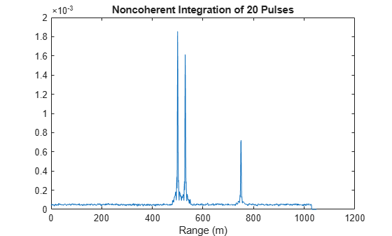
Integrate 20 pulses noncoherently.

intpulse = pulsint(resp(:,1:20),"noncoherent");
plot(rnggrid,abs(intpulse))
xlabel("Range (m)")
title("Noncoherent Integration of 20 Pulses")

Figure contains an axes object. The axes object with title Noncoherent Integration of 20 Pulses, xlabel Range (m) contains an object of type line.

Algorithms

expand all

References

[1] Richards, M. Fundamentals of Radar Signal Processing, 2nd ed. McGraw-Hill Professional Engineering, 2014.

[2] Richards, M., J. Scheer, and W. Holm, Principles of Modern Radar: Basic Principles. SciTech Publishing, 2010.

Extended Capabilities

expand all

Version History

Introduced in R2017a