Detect Anomalies in Industrial Machinery Using Three-Axis Vibration Data
Anomaly detection in machinery is often challenging because there is typically much more data available for normal behavior than for anomalous behavior. With two-class model training, this data imbalance results in a bias toward the larger class in the trained model.
An alternative approach to training models with both normal and anomalous data is to train models with only normal data, to such a degree of fidelity that the model detects any outlying data as anomalous.
This example shows how to use such an approach to detect anomalies in vibration data from industrial machinery, using models from machine learning and deep learning. The example assumes that machine data is anomalous before a maintenance event and normal after the event. This division allows normal-only data for training, and mixed data for testing, as the following figure shows.
The process includes the following steps:
1) Extract, rank, and select features from the raw vibration measurements using the Diagnostic Feature Designer app, using a reduced data set. Then, with app-generated code, generate the selected features for the full data set.
2) Partition this feature data into a training set and an independent test set. Then, from the training set, extract all features with the label 'After' to create a new training set that contains only normal data.
3) Retain the independent test set. This test set includes mixed data that can have either a 'Before'(anomalous) or an 'After' (normal) label.
4) Use the training set to train three different models (one-class SVM, isolation forest, and autoencoder) for anomaly detection.
5) Test each trained model using the test set to evaluate and compare how well the models identify whether each signal is anomalous or normal.
Download and Load Data Set
Download, unzip, and load the data set, which contains the labeled three-axis vibration measurements.
url = 'https://ssd.mathworks.com/supportfiles/predmaint/anomalyDetection3axisVibration/v1/vibrationData.zip';
websave('vibrationData.zip',url);
unzip('vibrationData.zip');
load("MachineData.mat")
head(trainData,3)
          ch1                 ch2                 ch3           label
    ________________    ________________    ________________    ______

    {70000×1 double}    {70000×1 double}    {70000×1 double}    Before
    {70000×1 double}    {70000×1 double}    {70000×1 double}    Before
    {70000×1 double}    {70000×1 double}    {70000×1 double}    Before
Data for each axis is stored in a separate column. Data collected before maintenance has the label Before, and is considered to be anomalous. Data collected after maintenance has the label 'After', and is considered to be normal.
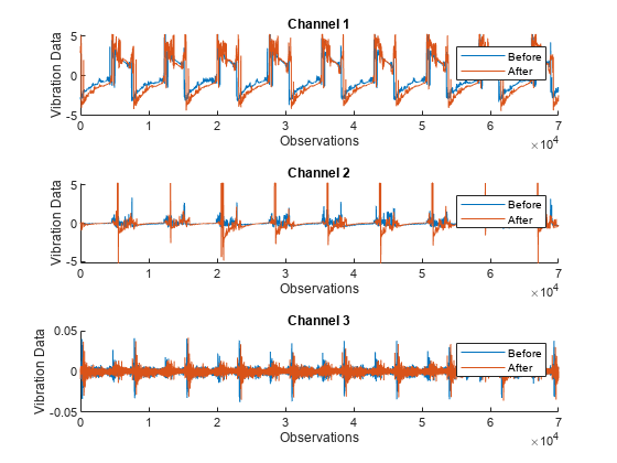
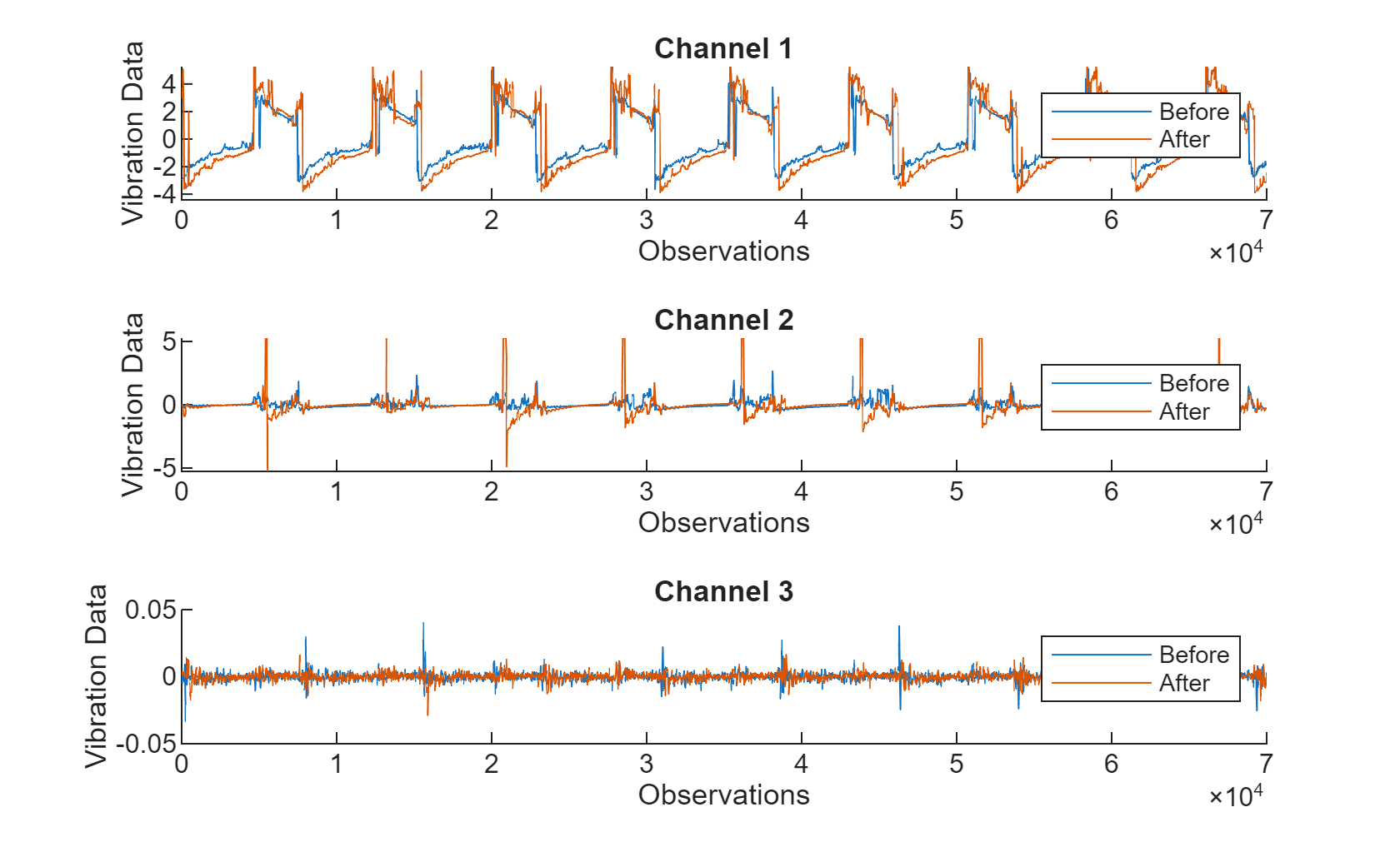
To better understand the data, visualize it before and after maintenance. Plot the vibration data for the fourth member of the ensemble and note that the plotted data for the two conditions looks different.
ensMember = 4;
helperPlotVibrationData(trainData, ensMember)
Extract Features with the Diagnostic Feature Designer App
Because raw data can be correlated and noisy, using raw data for training machine learning models is not very efficient. The Diagnostic Feature Designer app lets you interactively explore and preprocess your data, extract time and frequency domain features, and then rank the features to determine which are most effective for diagnosing faulty or otherwise anomalous systems. You can then export a function to extract the selected features from your data set programmatically. Open Diagnostic Feature Designer by typing diagnosticFeatureDesigner at the command prompt. For a tutorial on using Diagnostic Feature Designer, see Design Condition Indicators for Predictive Maintenance Algorithms.
Click the New Session button, select trainData as the source, and then set label as Condition Variable. The label variable identifies the condition of the machine for the corresponding data.

You can use Diagnostic Feature Designer to iterate on the features and rank them. The app creates a histogram view for all generated features to visualize the distribution for each label. For example, the following histograms show distributions of various features extracted from ch1. These histograms are derived from a much larger data set than the data set that you use in this example, in order to better illustrate the label-group separation. Because you are using a smaller data set, your results will look different.

Use the top four ranked features for each channel.
ch1: Crest Factor, Kurtosis, RMS, Stdch2: Mean, RMS, Skewness, Stdch3: Crest Factor, SINAD, SNR, THD
Export a function to generate the features from the Diagnostic Feature designer app and save it with the name generateFeatures. This function extracts the top 4 relevant features from each channel in the entire data set from the command line.
trainFeatures = generateFeatures(trainData);
head(trainFeatures(:,1:6))
    label     ch1_stats/Col1_CrestFactor    ch1_stats/Col1_Kurtosis    ch1_stats/Col1_RMS    ch1_stats/Col1_Std    ch2_stats/Col1_Mean
    ______    __________________________    _______________________    __________________    __________________    ___________________

    Before              2.2811                      1.8087                   2.3074                2.3071               -0.032332
    Before              2.3276                      1.8379                   2.2613                 2.261                -0.03331
    Before              2.3276                      1.8626                   2.2613                2.2612               -0.012052
    Before              2.8781                      2.1986                   1.8288                1.8285               -0.005049
    Before              2.8911                        2.06                   1.8205                1.8203              -0.0018988
    Before              2.8979                      2.1204                   1.8163                1.8162              -0.0044174
    Before              2.9494                        1.92                   1.7846                1.7844              -0.0067284
    Before              2.5106                      1.6774                   1.7513                1.7511              -0.0089548
Prepare Full Data Sets for Training and Testing
The data set you use to this point is only a small subset of a much larger data set to illustrate the process of feature extraction and selection. Training your algorithm on all available data yields the best performance. To this end, load the same 12 features as previously extracted from the larger data set of 17,642 signals.
load("FeatureEntire.mat")
head(featureAll(:,1:6))
label ch1_stats/Col1_CrestFactor ch1_stats/Col1_Kurtosis ch1_stats/Col1_RMS ch1_stats/Col1_Std ch2_stats/Col1_Mean
______ __________________________ _______________________ __________________ __________________ ___________________
Before 2.3683 1.927 2.2225 2.2225 -0.015149
Before 2.402 1.9206 2.1807 2.1803 -0.018269
Before 2.4157 1.9523 2.1789 2.1788 -0.0063652
Before 2.4595 1.8205 2.14 2.1401 0.0017307
Before 2.2502 1.8609 2.3391 2.339 -0.0081829
Before 2.4211 2.2479 2.1286 2.1285 0.011139
Before 3.3111 4.0304 1.5896 1.5896 -0.0080759
Before 2.2655 2.0656 2.3233 2.3233 -0.0049447
Use cvpartition to partition the data into a training set and an independent test set. Use the helperExtractLabeledData helper function to find all features corresponding to the label 'After' in the featureTrain variable.
rng(0) % set for reproducibility
idx = cvpartition(featureAll.label, 'holdout', 0.1);
featureTrain = featureAll(idx.training, :);
featureTest = featureAll(idx.test, :);
For each model, train on only the after-maintenance data, which is assumed to be normal. Extract only this data from featureTrain.
trueAnomaliesTest = featureTest.label;
featureNormal = featureTrain(featureTrain.label=='After', :);
Detect Anomalies with One-Class SVM
Support Vector Machines are powerful classifiers, and the variant that trains on only the normal data is used here. This model works well for identifying abnormalities that are "far" from the normal data. Train a one-class SVM model using the ocsvm function and the data for normal conditions.
rng(0) % For reproducibility
mdlOCSVM = ocsvm(featureNormal{:,2:13}, "ContaminationFraction", 0, "StandardizeData", true, "KernelScale", 4);
Validate the trained SVM model by using test data, which contains both normal and anomalous data.
featureTestNoLabels = featureTest(:, 2:end);
isanomalyOCSVM = isanomaly(mdlOCSVM, featureTestNoLabels.Variables, "ScoreThreshold", -0.4);
predOCSVM = categorical(isanomalyOCSVM, [1, 0], ["Anomaly", "Normal"]);

trueAnomaliesTest = renamecats(trueAnomaliesTest,["After","Before"], ["Normal","Anomaly"]);
figure;
confusionchart(trueAnomaliesTest, predOCSVM, Title="Anomaly Detection with One-class SVM", Normalization="row-normalized");
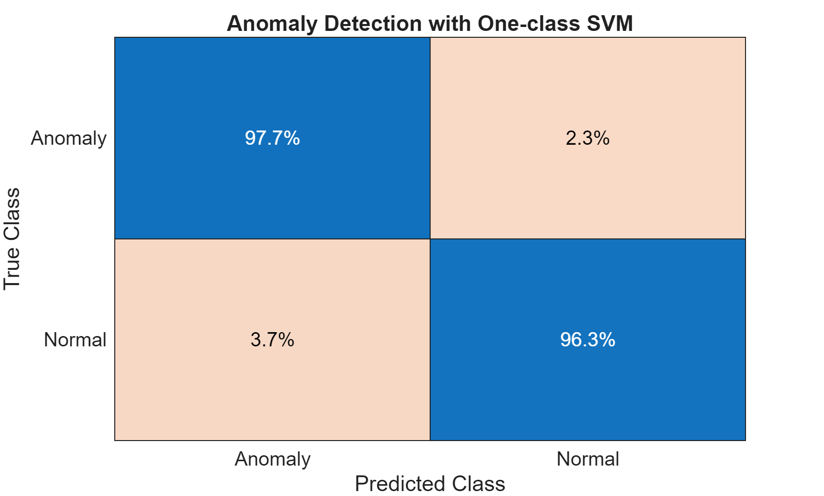
From the confusion matrix, you can see that the one-class SVM performs well, with high true positive identification and a very small misclassification percentage.
Detect Anomalies with Isolation Forest
The decision trees of an isolation forest isolate each observation in a leaf. How many decisions a sample passes through to get to its leaf is a measure of how difficult isolating it from the others is. The average depth of trees for a specific sample is used as their anomaly score and returned by iforest.
Train the isolation forest model on normal data only.
[mdlIF,~,scoreTrainIF] = iforest(featureNormal{:,2:13},'ContaminationFraction',0, 'NumLearners', 200, "NumObservationsPerLearner", 512);Validate the trained isolation forest model by using the test data. Visualize the performance of this model by using a confusion chart.
[isanomalyIF,scoreTestIF] = isanomaly(mdlIF,featureTestNoLabels.Variables, 'ScoreThreshold', 0.535);
predIF = categorical(isanomalyIF, [1, 0], ["Anomaly", "Normal"]);
figure;
confusionchart(trueAnomaliesTest,predIF,Title="Anomaly Detection with Isolation Forest",Normalization="row-normalized");

On this data, the isolation forest doesn't do as well as the one-class SVM. The performance of the isolation forest model can be further improved by additional data and hyper-parameter tuning activities.
Detect Anomalies with an Autoencoder Network
A fully connected autoencoder is used for reconstruction-based anomaly detection using the extracted feature data. In this workflow, the model is trained to encode normal data into a latent space and then reconstruct it as accurately as possible. Since it is optimized for reconstructing normal samples, it struggles to accurately reconstruct anomalous instances, leading to higher reconstruction errors. By setting a threshold on this error, anomalies can be detected.
Start by extracting features from the after maintenance data.
featuresAfter = helperExtractLabeledData(featureTrain, ...
   "After");
Construct the deep neural network and set the training options.
featureDimension = 12;

% Define Fully Connected network layers
layers = [
    featureInputLayer(featureDimension,Normalization="zscore")
    fullyConnectedLayer(32)
    layerNormalizationLayer
    reluLayer
    dropoutLayer
    fullyConnectedLayer(8)
    layerNormalizationLayer
    reluLayer
    fullyConnectedLayer(32)
    layerNormalizationLayer
    reluLayer
    fullyConnectedLayer(featureDimension)
    ];
% Set Training Options
options = trainingOptions('adam', ...
   'Plots', 'training-progress', ...
   'Metrics', 'rmse', ...
   'MiniBatchSize', 600,...
   'MaxEpochs',120, ...
   'Verbose',false);
The MaxEpochs training options parameter is set to 120. For higher validation accuracy, you can set this parameter to a larger number; However, the network might overfit.
Train the model using trainnet and specify mean-squared-error (mse) as the loss function.
net = trainnet(featuresAfter, featuresAfter, layers, "mse", options);
Visualize Model Behavior and Error on Validation Data
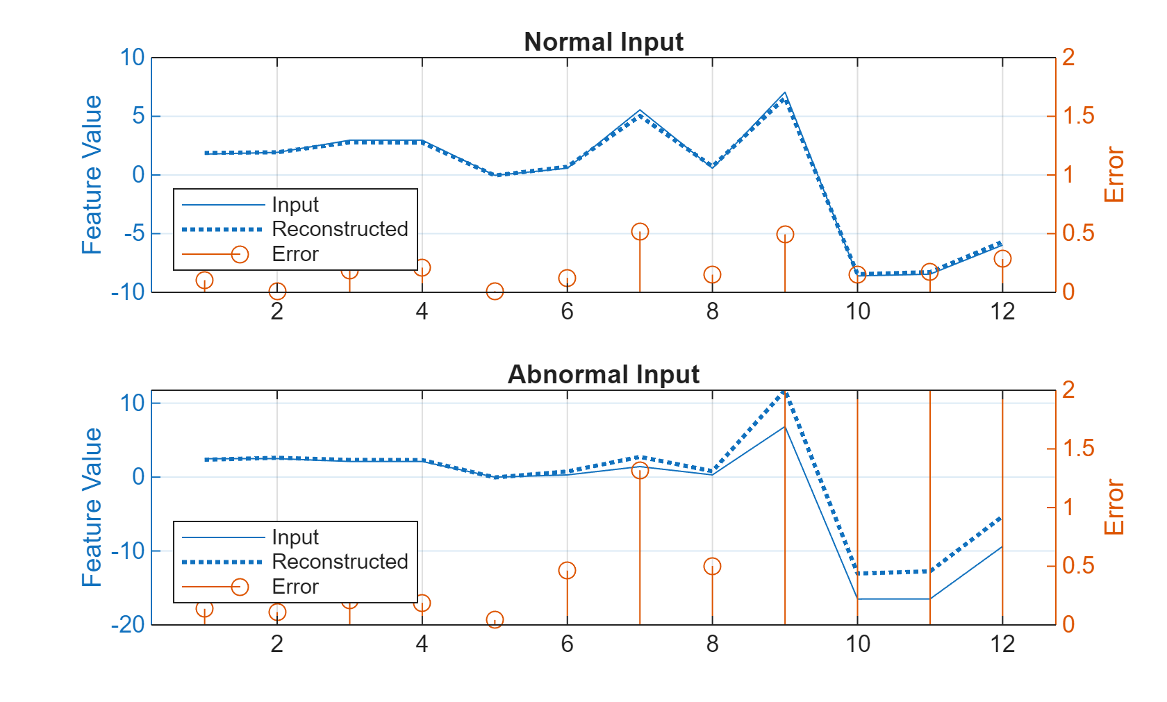
Extract and visualize a sample each from Anomalous and Normal condition. The following plots show the reconstruction errors of the deep neural network model for each of the 12 features (indicated on the X-axis). The reconstructed feature value is referred to as "Reconstructed" signal in the plot. In this sample, features 9, 10, 11, and 12 do not reconstruct well for the anomalous input and thus have high errors. You can use reconstruction errors to identify an anomaly.
testNormal = featureTest(1200, 2:end).Variables;
testAnomaly = featureTest(201, 2:end).Variables;

% Predict decoded signal for both
reconstructedNormal = predict(net,testNormal);
reconstructedAnomaly = predict(net,testAnomaly);

% Visualize
helperVisualizeModelBehavior(testNormal, testAnomaly, reconstructedNormal, reconstructedAnomaly)
Extract features for all the normal and anomalous data. Use the trained model to predict the selected 12 features for both before and after maintenance data. The following plots show the root mean square reconstruction error across the twelve features. The figure shows that the reconstruction error for the anomalous data is much higher than the normal data. This result is expected, since the network is trained on the normal data, so it better reconstructs similar signals.
% Extract data before maintenance
XTestBefore = helperExtractLabeledData(featureTest, "Before");

% Predict output before maintenance and calculate error
yHatBefore = minibatchpredict(net, XTestBefore, 'UniformOutput', true);
errorBefore = helperCalculateError(XTestBefore, yHatBefore);

% Extract data after maintenance
XTestAfter = helperExtractLabeledData(featureTest, "After");

% Predict output after maintenance and calculate error
yHatAfter = minibatchpredict(net, XTestAfter, 'UniformOutput', true);
errorAfter = helperCalculateError(XTestAfter, yHatAfter);

helperVisualizeError(errorBefore, errorAfter);

Identify Anomalies
Calculate the reconstruction error on the full validation data.
XTestAll = helperExtractLabeledData(featureTest, "All");

yHatAll = minibatchpredict(net, XTestAll, 'UniformOutput', true);
errorAll = helperCalculateError(XTestAll, yHatAll);
Define an anomaly as a point that has reconstruction error equal to the mean error across all observations of after maintenance data. This threshold was determined through previous experimentation and can be changed as required.
thresh = 1.2;
anomalies = errorAll > thresh*mean(errorAll);

helperVisualizeAnomalies(anomalies, errorAll, featureTest);
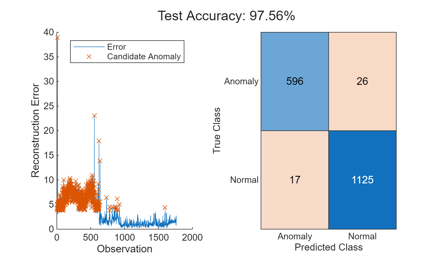
In this example, three different models are used to detect anomalies. All three models are able to detect anomalies with a high degree of accuracy and low misclassification percentages. The relative performance of the models can change if a different set of features are selected or if different hyperparameters are used for each model. Use the Diagnostic Feature Designer MATLAB app to further experiment with feature selection.
Supporting Functions
function E = helperCalculateError(X, Y)
% HELPERCALCULATEERROR calculates the rms error value between the
% inputs X, Y

E = zeros(height(X),1);
for i = 1:height(X)
    E(i,:) = sqrt(sum((Y(i,:) - X(i,:)).^2));
end
end

function helperVisualizeError(errorBefore, errorAfter)
% HELPERVISUALIZEERROR creates a plot to visualize the errors on detecting
% before and after conditions
figure("Color", "W")
tiledlayout("flow")

nexttile
plot(1:length(errorBefore), errorBefore, 'LineWidth',1.5), grid on
title(["Before Maintenance", ...
   sprintf("Mean Error: %.2f\n", mean(errorBefore))])
xlabel("Observations")
ylabel("Reconstruction Error")
ylim([0 15])

nexttile
plot(1:length(errorAfter), errorAfter, 'LineWidth',1.5), grid on,
title(["After Maintenance", ...
   sprintf("Mean Error: %.2f\n", mean(errorAfter))])
xlabel("Observations")
ylabel("Reconstruction Error")
ylim([0 15])

end

function helperVisualizeAnomalies(anomalies, errorAll, featureTest)
% HELPERVISUALIZEANOMALIES creates a plot of the detected anomalies
anomalyIdx = find(anomalies);
anomalyErr = errorAll(anomalies);

predAE = categorical(anomalies, [1, 0], ["Anomaly", "Normal"]);
trueAE = renamecats(featureTest.label,["Before","After"],["Anomaly","Normal"]);

acc = numel(find(trueAE == predAE))/numel(predAE)*100;
figure;
t = tiledlayout("flow");
title(t, "Test Accuracy: " + round(mean(acc),2) + "%");
nexttile
hold on
plot(errorAll)
plot(anomalyIdx, anomalyErr, 'x')
hold off
ylabel("Reconstruction Error")
xlabel("Observation")
legend("Error", "Candidate Anomaly")

nexttile
confusionchart(trueAE,predAE)

end

function helperVisualizeModelBehavior(normalData, abnormalData, reconstructedNorm, reconstructedAbNorm)
%HELPERVISUALIZEMODELBEHAVIOR Visualize model behavior on sample validation data

figure("Color", "W")
tiledlayout("flow")

nexttile()
hold on
colororder('default')
yyaxis left
plot(normalData')
plot(reconstructedNorm',":","LineWidth",1.5)
hold off
title("Normal Input")
grid on
ylabel("Feature Value")
yyaxis right
stem(abs(normalData' - reconstructedNorm'))
ylim([0 2])
ylabel("Error")
legend(["Input", "Reconstructed","Error"],"Location","southwest")

nexttile()
hold on
yyaxis left
plot(abnormalData)
plot(reconstructedAbNorm',":","LineWidth",1.5)
hold off
title("Abnormal Input")
grid on
ylabel("Feature Value")
yyaxis right
stem(abs(abnormalData' - reconstructedAbNorm'))
ylim([0 2])
ylabel("Error")
legend(["Input", "Reconstructed","Error"],"Location","southwest")

end

function X = helperExtractLabeledData(featureTable, label)
%HELPEREXTRACTLABELEDDATA Extract data from before or after operating
%conditions and re-format to support input to deep neural network

% Select data with label After
if label == "All"
   Xtemp = featureTable(:, 2:end).Variables;
else
   tF = featureTable.label == label;
   Xtemp = featureTable(tF, 2:end).Variables;
end

% Arrange data into cells
X = cell(length(Xtemp),1);
for i = 1:length(Xtemp)
   X{i,:} = Xtemp(i,:)';
end

X = horzcat(X{:})';
end
See Also
cvpartition | OneClassSVM | fitcsvm | iforest | Diagnostic Feature
Designer