Broken Rotor Fault Detection in AC Induction Motors Using Vibration and Electrical Signals

Open Live Script

This example shows how to detect failures in an AC induction motor. Typically, AC motors are driven by a three-phase power converter or an industrial power supply. Failures in the rotor bars of the motor can present themselves in various electrical and vibration signals collected from the system, including voltages and currents of each of the three phases and the acceleration and velocity signals in radial, axial, and tangential directions. Here, you use some of these signals in the Diagnostic Feature Designer app to extract features, which you then use to identify the number of broken rotor bars in the motor.

Data Set

The experimental workbench consists of a three-phase induction motor coupled with a direct-current machine, which works as a generator simulating the load torque, connected by a shaft containing a rotating torque meter. For more details about the workbench setup, see IEEE Broken Rotor Bar Database.

The data set contains electrical and mechanical signals from experiments on three-phase induction motors, using the experimental setup shown in the figure.

Electrical and vibration signals were collected from the system under the following health and loading conditions:

0, 1, 2, 3, and 4 broken rotor bars as the health condition
0.5, 1.0, 1.5, 2.0, 2.5, 3.0, 3.5, and 4.0 Nm torque as the load condition

Ten experiments were performed for each combination of health and loading condition. The following signals were acquired during each experiment:

Voltage of each phase ( $V_{a}$ , $V_{b}$ , $V_{c}$ )
Current draw of each phase ( $I_{a}$ , $I_{b}$ , $I_{c}$ )
Mechanical vibration speeds tangential to the housing ( ${Vib}_{carc}$ ) and base ( ${Vib}_{base}$ )
Mechanical vibration speed axial on the driven side ( ${Vib}_{axial}$ )
Mechanical vibration speeds radial on the driven side ( ${Vib}_{acpi}$ ) and nondriven side ( ${Vib}_{acpe}$ ).

For the full data set, visit IEEE Broken Rotor Bar Database, download the entire repository as a ZIP file, and save it in the same directory as this Live Script.

% Remove this comment when using the original data set.
% filename = "banco de dados experimental.zip";

Alternatively, you can use a reduced data set from the MathWorks repository. This data set contains two experiments per operating condition.

% Comment out this section when using the original data set.
filename = "experimental_database_short.zip";
if ~exist(filename,'file')
  url = "https://ssd.mathworks.com/supportfiles/predmaint/broken-rotor-bar-fault-data/" + filename;
  websave(filename,url);
end

Extract the compressed data files into the current folder.

unzip(filename)

Extract Ensemble Member Data

Convert the original motor data files into individual ensemble member data files for all combinations of health condition, load torque, and experiment index. The files are saved to a target folder and used by the fileEnsembleDatastore object in the Diagnostic Feature Designer app for data processing and feature extraction.

You can change the amount of experiments per operating condition to use in the ensemble data. If you use the reduced data set, use two experiments; otherwise, you can use up to 10.

numExperiments = 2; % Up to a maximum of 10 if using the original data set

The unzipped files of the original data set are associated with different numbers of broken rotor bars. Create bookkeeping variables to associate the original data files with the corresponding number of broken rotor bars.

% Names of the original data files restored from the zip archive.
files = [ ...
  "struct_rs_R1.mat", ...
  "struct_r1b_R1.mat", ...
  "struct_r2b_R1.mat", ...
  "struct_r3b_R1.mat", ...
  "struct_r4b_R1.mat", ...
  ];

% Rotor conditions (that is, number of broken bars) corresponding to original data files.
health = [
  "healthy", ...
  "broken_bar_1", ...
  "broken_bar_2", ...
  "broken_bar_3", ...
  "broken_bar_4", ...
  ];

Fs_vib = 7600; % Sampling frequency of vibration signals in Hz.
Fs_elec = 50000; % Sampling frequency of electrical signals in Hz.

Create a target folder to store the ensemble member data files that you generate next.

folder = 'data_files';
if ~exist(folder, 'dir')
  mkdir(folder);
end

Iterate over the original data files, where each file corresponds to a given number of broken rotor bars, and construct individual ensemble member data files for each combination of load and number of broken rotor bars.

% Iterate over the number of broken rotor bars.
for i = 1:numel(health)
  fprintf('Processing data file %s\n', files(i))

  % Load the original data set stored as a struct.
  S = load(files(i));
  fields = fieldnames(S);
  dataset = S.(fields{1});

  loadLevels = fieldnames(dataset);
  % Iterate over load (torque) levels in each data set.
  for j = 1:numel(loadLevels)
    experiments = dataset.(loadLevels{j});
    data = struct;

    % Iterate over the given number of experiments for each load level.
    for k = 1:numExperiments
      signalNames = fieldnames(experiments(k));
      % Iterate over the signals in each experimental data set.
      for l = 1:numel(signalNames)
        % Experimental (electrical and vibration) data
        data.(signalNames{l}) = experiments(k).(signalNames{l});
      end

      % Operating conditions
      data.Health = health(i);
      data.Load = string(loadLevels{j});

      % Constant parameters
      data.Fs_vib = Fs_vib;
      data.Fs_elec = Fs_elec;

      % Save memberwise data.
      name = sprintf('rotor%db_%s_experiment%02d',  i-1, loadLevels{j}, k);
      fprintf('\tCreating the member data file %s.mat\n', name)
      filename = fullfile(pwd, folder, name);
      save(filename, '-v7.3', '-struct', 'data'); % Save fields as individual variables.
    end
  end
end

Processing data file struct_rs_R1.mat

	Creating the member data file rotor0b_torque05_experiment01.mat
	Creating the member data file rotor0b_torque05_experiment02.mat
	Creating the member data file rotor0b_torque10_experiment01.mat
	Creating the member data file rotor0b_torque10_experiment02.mat
	Creating the member data file rotor0b_torque15_experiment01.mat
	Creating the member data file rotor0b_torque15_experiment02.mat
	Creating the member data file rotor0b_torque20_experiment01.mat
	Creating the member data file rotor0b_torque20_experiment02.mat
	Creating the member data file rotor0b_torque25_experiment01.mat
	Creating the member data file rotor0b_torque25_experiment02.mat
	Creating the member data file rotor0b_torque30_experiment01.mat
	Creating the member data file rotor0b_torque30_experiment02.mat
	Creating the member data file rotor0b_torque35_experiment01.mat
	Creating the member data file rotor0b_torque35_experiment02.mat
	Creating the member data file rotor0b_torque40_experiment01.mat
	Creating the member data file rotor0b_torque40_experiment02.mat

Processing data file struct_r1b_R1.mat

	Creating the member data file rotor1b_torque05_experiment01.mat
	Creating the member data file rotor1b_torque05_experiment02.mat
	Creating the member data file rotor1b_torque10_experiment01.mat
	Creating the member data file rotor1b_torque10_experiment02.mat
	Creating the member data file rotor1b_torque15_experiment01.mat
	Creating the member data file rotor1b_torque15_experiment02.mat
	Creating the member data file rotor1b_torque20_experiment01.mat
	Creating the member data file rotor1b_torque20_experiment02.mat
	Creating the member data file rotor1b_torque25_experiment01.mat
	Creating the member data file rotor1b_torque25_experiment02.mat
	Creating the member data file rotor1b_torque30_experiment01.mat
	Creating the member data file rotor1b_torque30_experiment02.mat
	Creating the member data file rotor1b_torque35_experiment01.mat
	Creating the member data file rotor1b_torque35_experiment02.mat
	Creating the member data file rotor1b_torque40_experiment01.mat
	Creating the member data file rotor1b_torque40_experiment02.mat

Processing data file struct_r2b_R1.mat

	Creating the member data file rotor2b_torque05_experiment01.mat
	Creating the member data file rotor2b_torque05_experiment02.mat
	Creating the member data file rotor2b_torque10_experiment01.mat
	Creating the member data file rotor2b_torque10_experiment02.mat
	Creating the member data file rotor2b_torque15_experiment01.mat
	Creating the member data file rotor2b_torque15_experiment02.mat
	Creating the member data file rotor2b_torque20_experiment01.mat
	Creating the member data file rotor2b_torque20_experiment02.mat
	Creating the member data file rotor2b_torque25_experiment01.mat
	Creating the member data file rotor2b_torque25_experiment02.mat
	Creating the member data file rotor2b_torque30_experiment01.mat
	Creating the member data file rotor2b_torque30_experiment02.mat
	Creating the member data file rotor2b_torque35_experiment01.mat
	Creating the member data file rotor2b_torque35_experiment02.mat
	Creating the member data file rotor2b_torque40_experiment01.mat
	Creating the member data file rotor2b_torque40_experiment02.mat

Processing data file struct_r3b_R1.mat

	Creating the member data file rotor3b_torque05_experiment01.mat
	Creating the member data file rotor3b_torque05_experiment02.mat
	Creating the member data file rotor3b_torque10_experiment01.mat
	Creating the member data file rotor3b_torque10_experiment02.mat
	Creating the member data file rotor3b_torque15_experiment01.mat
	Creating the member data file rotor3b_torque15_experiment02.mat
	Creating the member data file rotor3b_torque20_experiment01.mat
	Creating the member data file rotor3b_torque20_experiment02.mat
	Creating the member data file rotor3b_torque25_experiment01.mat
	Creating the member data file rotor3b_torque25_experiment02.mat
	Creating the member data file rotor3b_torque30_experiment01.mat
	Creating the member data file rotor3b_torque30_experiment02.mat
	Creating the member data file rotor3b_torque35_experiment01.mat
	Creating the member data file rotor3b_torque35_experiment02.mat
	Creating the member data file rotor3b_torque40_experiment01.mat
	Creating the member data file rotor3b_torque40_experiment02.mat

Processing data file struct_r4b_R1.mat

	Creating the member data file rotor4b_torque05_experiment01.mat
	Creating the member data file rotor4b_torque05_experiment02.mat
	Creating the member data file rotor4b_torque10_experiment01.mat
	Creating the member data file rotor4b_torque10_experiment02.mat
	Creating the member data file rotor4b_torque15_experiment01.mat
	Creating the member data file rotor4b_torque15_experiment02.mat
	Creating the member data file rotor4b_torque20_experiment01.mat
	Creating the member data file rotor4b_torque20_experiment02.mat
	Creating the member data file rotor4b_torque25_experiment01.mat
	Creating the member data file rotor4b_torque25_experiment02.mat
	Creating the member data file rotor4b_torque30_experiment01.mat
	Creating the member data file rotor4b_torque30_experiment02.mat
	Creating the member data file rotor4b_torque35_experiment01.mat
	Creating the member data file rotor4b_torque35_experiment02.mat
	Creating the member data file rotor4b_torque40_experiment01.mat
	Creating the member data file rotor4b_torque40_experiment02.mat

Construct File Ensemble Datastore

Create a file ensemble datastore for the data stored in the MAT-files, and configure it with functions that interact with the software to read from and write to the datastore.

location = fullfile(pwd, folder);
ens = fileEnsembleDatastore(location,'.mat');

Before you can interact with data in the ensemble, you must create functions that tell the software how to process the data files to read variables into the MATLAB workspace and to write data back to the files. For this example, use the following supplied functions.

readMemberData — Extract requested variables stored in the file. The function returns a table row containing one table variable for each requested variable.
writeMemberData — Take a structure and write its variables to a data file as individual stored variables.

ens.ReadFcn = @readMemberData;
ens.WriteToMemberFcn = @writeMemberData;

Finally, set properties of the ensemble to identify data variables, condition variables, and the variables selected to read. These variables include ones that are not in the original data set but rather specified and constructed by readMemberData: Vib_acpi_env, the band-pass filtered radial vibration signal, and Ia_env_ps, the band-pass filtered envelope spectrum of the first-phase current signal. Diagnostic Feature Designer can read synthetic signals such as these as well.

ens.DataVariables = [...
  "Va"; "Vb"; "Vc"; "Ia"; "Ib"; "Ic"; ...
  "Vib_acpi"; "Vib_carc"; "Vib_acpe"; "Vib_axial"; "Vib_base"; "Trigger"];
ens.ConditionVariables = ["Health"; "Load"];
ens.SelectedVariables = ["Ia"; "Vib_acpi"; "Health"; "Load"];

% Add synthetic signals and spectra generated directly in the readMemberData
% function.
ens.DataVariables = [ens.DataVariables; "Vib_acpi_env"; "Ia_env_ps"];
ens.SelectedVariables = [ens.SelectedVariables; "Vib_acpi_env"; "Ia_env_ps"];

Examine the ensemble. The functions and the variable names are assigned to the appropriate properties.

ens

ens = 
  fileEnsembleDatastore with properties:

                 ReadFcn: @readMemberData
        WriteToMemberFcn: @writeMemberData
           DataVariables: [14×1 string]
    IndependentVariables: [0×0 string]
      ConditionVariables: [2×1 string]
       SelectedVariables: [6×1 string]
                ReadSize: 1
              NumMembers: 80
          LastMemberRead: [0×0 string]
                   Files: [80×1 string]

Examine a member of the ensemble and confirm that the desired variables are read or generated.

T = read(ens)

T=1×6 table
            Ia                  Vib_acpi            Vib_acpi_env          Ia_env_ps         Health         Load   
    ___________________    __________________    __________________    ________________    _________    __________

    {50001×1 timetable}    {7601×1 timetable}    {7601×1 timetable}    {25001×2 double}    "healthy"    "torque05"

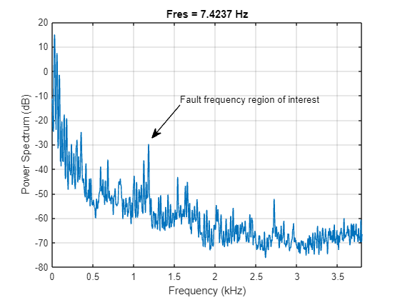
From the power spectrum of one of the vibration signals, Vib_acpi, observe that there are frequency components of interest in the [900 1300] Hz region. These components are a primary reason why you use readMemberData to compute the band-pass filtered variables - Vib_acpi_env and Ia_env_ps.

% Power spectrum of vibration signal, Vib_acpi
vib = T.Vib_acpi{1};
pspectrum(vib.Data, Fs_vib);
annotation("textarrow", [0.45 0.38], [0.65 0.54], "String", "Fault frequency region of interest")

The envelope of signals after band-pass filtering them can help reveal demodulated signals containing behavior related to the health of the system.

% Envelop of vibration signal
y = bandpass(vib.Data, [900 1300], Fs_vib);
envelope(y)
axis([0 800 -0.5 0.5])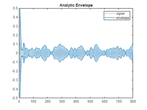

Import Data into Diagnostic Feature Designer App

Open the Diagnostic Feature Designer app using the following command.

app = diagnosticFeatureDesigner;

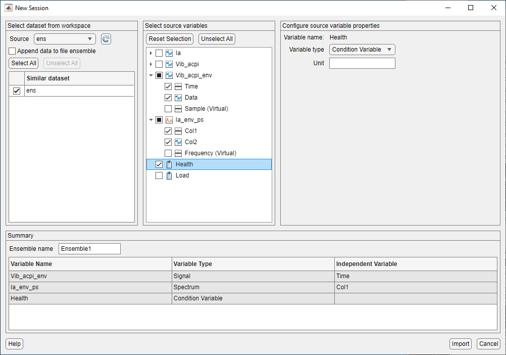
You can then import the file ensemble datastore into the app by clicking the New Session button and selecting the ens variable from the list.

Once preliminary data is read by the app, make sure to uncheck the Append data to file ensemble option if you do not want to write new features or data back to the ensemble member files. When you are working with the smaller data set in this example, generating new features directly in memory is faster, so uncheck the option.

Alternatively, if the whole data set is small enough to fit into your computer's memory, then you can read it into a table object using the following command then import the table into the app directly.

% Working with in-memory data in the app. This may take a couple of minutes to
% run.
T = readall(ens)

T=80×6 table
            Ia                  Vib_acpi            Vib_acpi_env          Ia_env_ps         Health         Load   
    ___________________    __________________    __________________    ________________    _________    __________

    {50001×1 timetable}    {7601×1 timetable}    {7601×1 timetable}    {25001×2 double}    "healthy"    "torque05"
    {50001×1 timetable}    {7601×1 timetable}    {7601×1 timetable}    {25001×2 double}    "healthy"    "torque05"
    {50001×1 timetable}    {7601×1 timetable}    {7601×1 timetable}    {25001×2 double}    "healthy"    "torque10"
    {50001×1 timetable}    {7601×1 timetable}    {7601×1 timetable}    {25001×2 double}    "healthy"    "torque10"
    {50001×1 timetable}    {7601×1 timetable}    {7601×1 timetable}    {25001×2 double}    "healthy"    "torque15"
    {50001×1 timetable}    {7601×1 timetable}    {7601×1 timetable}    {25001×2 double}    "healthy"    "torque15"
    {50001×1 timetable}    {7601×1 timetable}    {7601×1 timetable}    {25001×2 double}    "healthy"    "torque20"
    {50001×1 timetable}    {7601×1 timetable}    {7601×1 timetable}    {25001×2 double}    "healthy"    "torque20"
    {50001×1 timetable}    {7601×1 timetable}    {7601×1 timetable}    {25001×2 double}    "healthy"    "torque25"
    {50001×1 timetable}    {7601×1 timetable}    {7601×1 timetable}    {25001×2 double}    "healthy"    "torque25"
    {50001×1 timetable}    {7601×1 timetable}    {7601×1 timetable}    {25001×2 double}    "healthy"    "torque30"
    {50001×1 timetable}    {7601×1 timetable}    {7601×1 timetable}    {25001×2 double}    "healthy"    "torque30"
    {50001×1 timetable}    {7601×1 timetable}    {7601×1 timetable}    {25001×2 double}    "healthy"    "torque35"
    {50001×1 timetable}    {7601×1 timetable}    {7601×1 timetable}    {25001×2 double}    "healthy"    "torque35"
    {50001×1 timetable}    {7601×1 timetable}    {7601×1 timetable}    {25001×2 double}    "healthy"    "torque40"
    {50001×1 timetable}    {7601×1 timetable}    {7601×1 timetable}    {25001×2 double}    "healthy"    "torque40"
      ⋮

Envelope Signal Data

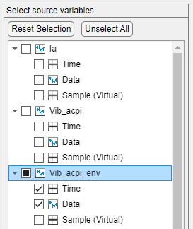
Select the time-domain signals to import in the tree view of the New Session dialog. Here, you only use the synthetic signals, so uncheck Ia and Vib_acpi. Keep the envelope of the radial vibration speed on the driven side Vib_acpi_env checked; you do not need to modify it otherwise.

Envelope Spectrum Data

Select the frequency-domain data to import. Keep the envelope spectrum of Phase A current Ia_env_ps selected and change its Variable type to Spectrum.

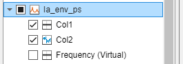
Specify Col1 as an independent (frequency) variable with a corresponding 50 kHz sampling frequency.

Condition Variables

Finally, the condition variable of interest for fault classification is the Health variable, which corresponds to the number of broken rotor bars in the experiments. Ensure that its Variable type is Condition Variable.

Confirm the final ensemble specification and click Import.

Once the file ensemble is imported, you can visualize the data by creating Signal Trace plots and grouping the plot colors based on the Health status of the experimental data. Note that reading all members of the file ensemble to produce plots and process the data might be time-consuming depending on the size and number of the data files that need to be read.

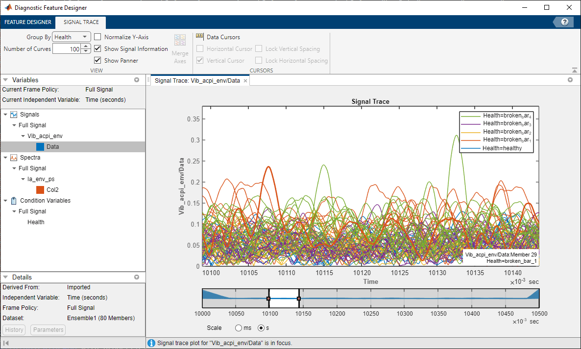
Note that the getSignal function used in readMemberData reads a portion of the signals from each member file after the initial transients due to motor startup have died down. In this case, the function loads only the data between 10.0 and 11.0 seconds

Create Predictive Features

The Auto Features option is a fast way of creating a large number of features from available signals and ranking them according to their power in separating various health classes. For the imported time-domain signal Vib_acpi_env, apply the Auto Features option by selecting the signal in the Data Browser tree and clicking Auto Features on the Feature Designer tab.

Clicking Compute generates a large number of features automatically and ranks them according their importance with respect to the One-way ANOVA criterion. This computation might take a few minutes to run.

For generating features from envelope spectrum data, a more manual approach can yield more precise results. Select the Ia_env_ps signal in the Data Browser, and select Custom Faults Features under the Frequency-Domain Features menu. Select fault bands around a fundamental frequency of 60 Hz and its first 6 harmonics along with a sideband of 30 Hz to cover most of the spectral peaks in the envelope spectra. Use a fault band width of 10 Hz. Click Apply to generate features.

You have now generated a large number of features from the various electrical and vibration signals of the AC motor system.

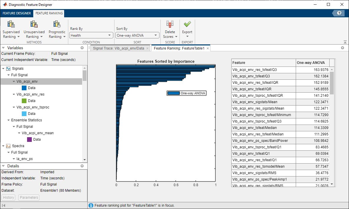
Rank Features

This process allows you to quickly create about 150 features both manually and automatically. The final ranking table indicates that the first 10 to 15 features, based on One-way ANOVA ranking, help classify the motors according to the number of broken rotor bars in them.

When fault bands and their corresponding names are difficult to identify, use the Peak Frequency feature to identify the corresponding fault band frequency/region.

Export Features to Classification Learner App and Build a Tree Model

Export the top features from the Diagnostic Feature Designer app using Export > Export Features To Classification Learner on the Feature Ranking tab. Change Select top features to 10.

Click Export to start the Classification Learner app. The New Session from File dialog is populated correctly, so click Start Session to load the feature data into the app.

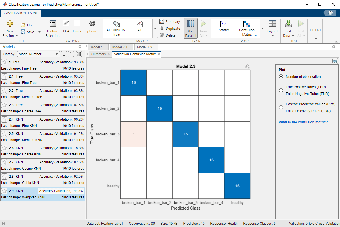
Click Train All on the Classification Learner tab to obtain a Tree model that achieves about 94% accuracy in classifying the motor faults (that is, the number of broken rotor bars) using the 10 features imported into the app.

To generate a selection of fast-fitting models, All Quick-To-Train from the Models gallery, click Train All. The weighted KNN model number 2.9 in the figure is able to classify broken rotor faults with about 98% accuracy.

Supporting Functions

The WriteToMemberFcn property of the fileEnsembleDatastore object stores the handle of the function responsible for adding new data to each member of the ensemble. The Diagnostic Feature Designer app uses this function to save new processed data and extracted features.

function writeMemberData(filename, data)
% Write data into the fileEnsembleDatastore.
%
% Inputs:
%  filename - a string for the file name to write
%  data     - a data structure to write to the file

% Save fields as individual variables.
save(filename, '-append', '-struct', 'data');
end

The function stored in the ReadFcn property of the fileEnsembleDatastore object reads member data from ensemble member files. The Diagnostic Feature Designer app uses this function to read signals, spectra, and features. You can also use this function to create synthetic signals on the fly that can be used in the app.

function T = readMemberData(filename, variables)
% Read variables from a fileEnsembleDatastore
%
% Inputs:
%  filename  - file to read, specified as a string
%  variables - variable names to read, specified as a string array
%              Variables must be a subset of SelectedVariables specified in
%              the fileEnsembleDatastore.
% Output:
%  T         - a table with a single row

mfile = matfile(filename); % Allows partial loading

% Read condition variables directly from the top-level structure fields
T = table();
for i = 1:numel(variables)
  var = variables(i);

  switch var
    case {'Health', 'Load'}
      % Condition variables
      val = mfile.(var);
    case {'Va', 'Vb', 'Vc', 'Ia', 'Ib', 'Ic'}
      % Electrical signals
      val = getSignal(mfile, var, mfile.Fs_elec);
    case {'Vib_acpi', 'Vib_carc', 'Vib_acpe', 'Vib_axial', 'Vib_base', 'Trigger'}
      % Vibration signals
      val = getSignal(mfile, var, mfile.Fs_vib);
    case {'Vib_acpi_env'}
      % Synthetic envelope signals for vibration data
      sig = regexprep(var, '_env', '');
      TT = getSignal(mfile, sig, mfile.Fs_vib);
      % Envelope of band-pass filtered signal
      y = bandpass(TT.Data, [900 1300], mfile.Fs_vib);
      yUpper = envelope(y);
      val = timetable(yUpper, 'VariableNames', "Data", 'RowTimes', TT.Time);
    case {'Ia_env'}
      % Synthetic envelope signals for electrical data
      sig = regexprep(var, '_env', '');
      TT = getSignal(mfile, sig, mfile.Fs_elec);
      % Envelope of band-pass filtered signal
      y = bandpass(TT.Data, [900 1300], mfile.Fs_elec);
      yUpper = envelope(y);
      val = timetable(yUpper, 'VariableNames', "Data", 'RowTimes', TT.Time);
    case {'Ia_env_ps'}
      % Synthetic envelope spectra for electrical data
      sig = regexprep(var, '_env_ps', '');
      TT = getSignal(mfile, sig, mfile.Fs_elec);
      % Envelope spectrum of band-pass filtered signal
      [ES,F] = envspectrum(TT, 'Method', 'hilbert', 'Band', [900 1300]);
      val = [F,ES];
    otherwise
      % Other features and signals.
      val = mfile.(var);
  end

  if numel(val) > 1
    val = {val};
  end

  % Add the data to the output table, using the variable name.
  T.(var) = val;
end
end

When the original signal is longer than what is needed to extract useful features from it, you can use the following helper function to extract a shorter portion of the full signal from the member data.

function TT = getSignal(mfile, signame, Fs)
% Extract a 1.0 second portion of the signal after 10 seconds of measurements.
signame = char(signame);
n = size(mfile, signame, 1);
t = (0:n-1)' / Fs;
I = find((t >= 10.0) & (t <= 11.0)); % 1.0 sec of data
TT = timetable(mfile.(signame)(I,1), 'VariableNames', "Data", 'RowTimes', seconds(t(I)));
end

References

Treml, Aline Elly, Rogério Andrade Flauzino, Marcelo Suetake, and Narco Afonso Ravazzoli Maciejewski. "Experimental database for detecting and diagnosing rotor broken bar in a threephase induction motor." IEEE Dataport, updated September 24, 2020, https://dx.doi.org/10.21227/fmnm-bn95.