Train TD3 Agent for PMSM Control

This example demonstrates speed control of a permanent magnet synchronous motor (PMSM) using a twin delayed deep deterministic policy gradient (TD3) agent.

The goal of this example is to show that you can use reinforcement learning as an alternative to linear controllers, such as PID controllers, to control the speed of PMSM systems. Linear controllers often do not produce good tracking performance outside the region in which the plant can be approximated with a linear system. In such cases, reinforcement learning provides a nonlinear control alternative.

Load the parameters for this example.

sim_data

### The Lq is observed to be lower than Ld. ### 
### Using the lower of these two for the Ld (internal variable)  ### 
### and higher of these two for the Lq (internal variable) for computations. ###
### The Lq is observed to be lower than Ld. ### 
### Using the lower of these two for the Ld (internal variable)  ### 
### and higher of these two for the Lq (internal variable) for computations. ###
             model: 'Maxon-645106'
                sn: '2295588'
                 p: 7
                Rs: 0.2930
                Ld: 8.7678e-05
                Lq: 7.7724e-05
                Ke: 5.7835
                 J: 8.3500e-05
                 B: 7.0095e-05
           I_rated: 7.2600
          QEPSlits: 4096
            N_base: 3476
             N_max: 4300
            FluxPM: 0.0046
           T_rated: 0.3471
    PositionOffset: 0.1650

               model: 'BoostXL-DRV8305'
                  sn: 'INV_XXXX'
                V_dc: 24
              I_trip: 10
              Rds_on: 0.0020
              Rshunt: 0.0070
       CtSensAOffset: 2295
       CtSensBOffset: 2286
       CtSensCOffset: 2295
             ADCGain: 1
         EnableLogic: 1
        invertingAmp: 1
          ISenseVref: 3.3000
    ISenseVoltPerAmp: 0.0700
           ISenseMax: 21.4286
             R_board: 0.0043
     CtSensOffsetMax: 2500
     CtSensOffsetMin: 1500

                 model: 'LAUNCHXL-F28379D'
                    sn: '123456'
         CPU_frequency: 200000000
         PWM_frequency: 5000
    PWM_Counter_Period: 20000
              ADC_Vref: 3
          ADC_MaxCount: 4095
         SCI_baud_rate: 12000000

    V_base: 13.8564
    I_base: 21.4286
    N_base: 3476
    T_base: 1.0249
    P_base: 445.3845

Open the Simulink model.

mdl = "mcb_pmsm_foc_sim_RL";
open_system(mdl)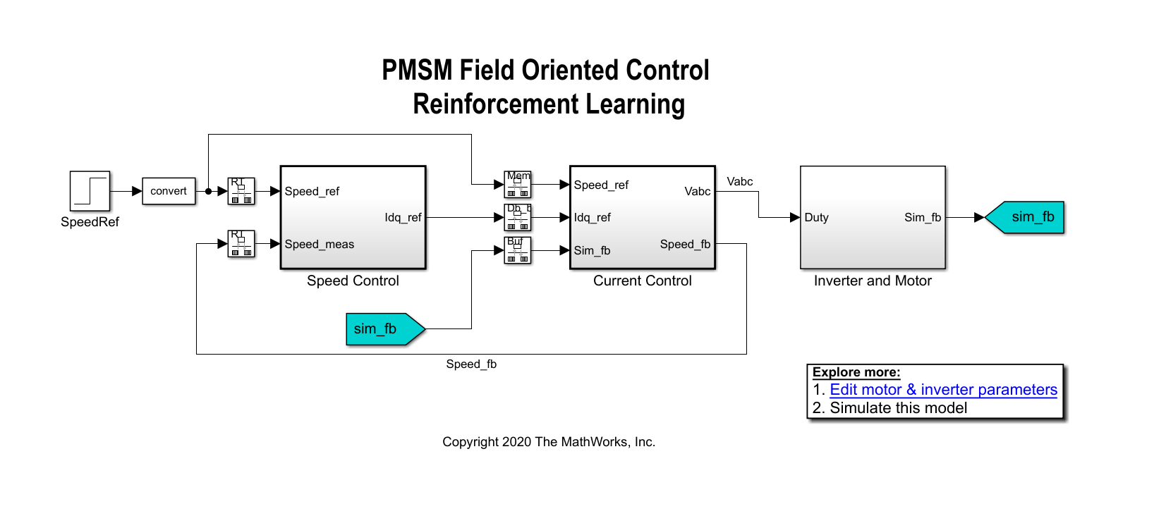

In a linear control version of this example, you can use PI controllers in both the speed and current control loops. An outer-loop PI controller can control the speed while two inner-loop PI controllers control the d-axis and q-axis currents. The overall goal is to track the reference speed in the Speed_Ref signal. This example uses a reinforcement learning agent to control the currents in the inner control loop while a PI controller controls the outer loop.

Create Environment Interface

The environment in this example consists of the PMSM system, excluding the inner-loop current controller, which is the reinforcement learning agent. To view the interface between the reinforcement learning agent and the environment, open the Closed Loop Control subsystem.

open_system(mdl + ...
    "/Current Control/Control_System/Closed Loop Control")

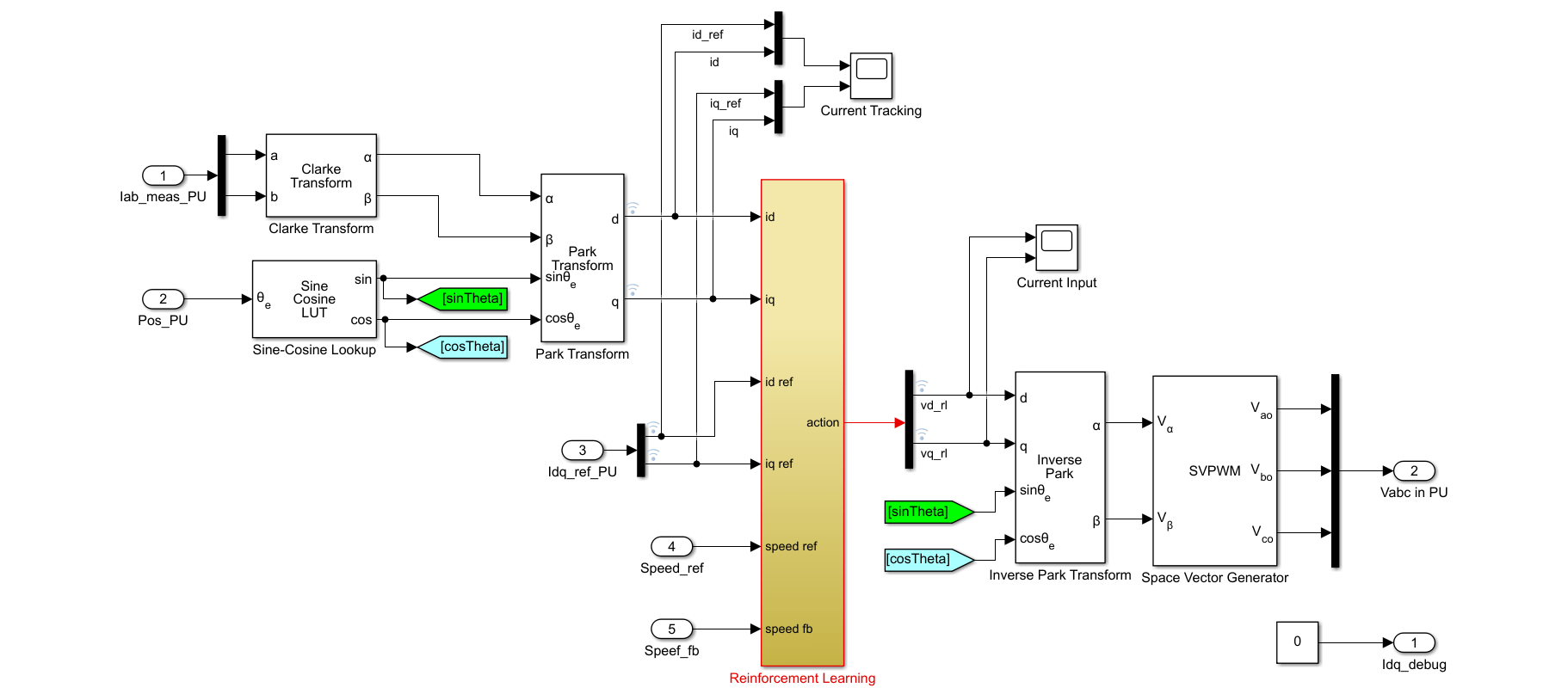
The Reinforcement Learning subsystem contains an RL Agent block, the creation of the observation vector, and the reward calculation.

For this environment:

• The observations are the outer-loop reference speed Speed_ref, speed feedback Speed_fb, d-axis and q-axis currents and errors ($\mathrm{id}$, $\mathrm{iq}$, ${\mathrm{id}}_{\mathrm{error}}$ and ${\mathrm{iq}}_{\mathrm{error}}$), and the error integrals.

• The actions from the agent are the voltages vd_rl and vq_rl.

• The sample time of the agent is 2e-4 seconds. The inner-loop control occurs at a different sample time than the outer loop control.

• The simulation runs for 5000 time steps unless it is terminated early when the ${\mathrm{iq}}_{\mathrm{ref}}$ signal is saturated at 1.

• The reward at each time step is:

$${\mathit{r}}_{\mathit{t}}=-\left({\mathit{Q}}_1*{{\mathrm{id}}_{\mathrm{error}}}^2+{\mathit{Q}}_2*{{\mathrm{iq}}_{\mathrm{error}}}^2+\mathit{R}*\sum _{\mathit{j}}{{{\mathit{u}}^{\mathit{j}}}_{\mathit{t}-1}}^2\right)-100\mathit{d}$$

Here, ${\mathit{Q}}_1={\mathit{Q}}_2=5$, and $\mathit{R}=0.1$ are constants, ${\mathrm{id}}_{\mathrm{error}}$ is the d-axis current error, ${\mathrm{iq}}_{\mathrm{error}}$ is the q-axis current error, ${{\mathit{u}}^{\mathit{j}}}_{\mathit{t}-1}$ are the actions from the previous time step, and $\mathit{d}$ is a flag that is equal to 1 when the simulation is terminated early.

Create the observation and action specifications for the environment. For information on creating continuous specifications, see rlNumericSpec.

% Create observation specifications.
numObs = 8;
obsInfo = rlNumericSpec( ...
    [numObs 1], ...
    DataType=dataType);
obsInfo.Name = "observations";
obsInfo.Description = "Error and reference signal";

% Create action specifications.
numAct = 2;
actInfo = rlNumericSpec([numAct 1], "DataType", dataType); 
actInfo.Name = "vqdRef";

Create the Simulink environment interface using the observation and action specifications. For more information on creating Simulink environments, see rlSimulinkEnv.

agentblk = "mcb_pmsm_foc_sim_RL/Current Control/" + ... 
   "Control_System/Closed Loop Control/" + ... 
   "Reinforcement Learning/RL Agent";

env = rlSimulinkEnv(mdl, agentblk, obsInfo, actInfo);

Provide a reset function for this environment using the ResetFcn parameter. At the beginning of each training episode, the resetPMSM function randomly initializes the final value of the reference speed in the SpeedRef block to 695.4 rpm (0.2 pu), 1390.8 rpm (0.4 pu), 2086.2 rpm (0.6 pu), or 2781.6 rpm (0.8 pu).

env.ResetFcn = @resetPMSM;

Create Agent

The agent used in this example is a twin-delayed deep deterministic policy gradient (TD3) agent. TD3 agents use two parametrized Q-value function approximators to estimate the value (that is the expected cumulative long-term reward) of the policy.

To model the parametrized Q-value function within both critics, use a neural network with two inputs (the observation and action) and one output (the value of the policy when taking a given action from the state corresponding to a given observation). For more information on TD3 agents, see Twin-Delayed Deep Deterministic (TD3) Policy Gradient Agents.

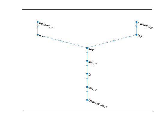
Define each network path as an array of layer objects. Assign names to the input and output layers of each path. These names allow you to connect the paths and then later explicitly associate the network input and output layers with the appropriate environment channel.

% State input path
statePath = [
    featureInputLayer(numObs, Name="StateInLyr")
    fullyConnectedLayer(64, Name="fc1")
    ];

% Action input path
actionPath = [
    featureInputLayer(numAct, Name="ActionInLyr")
    fullyConnectedLayer(64, Name="fc2")
    ];

% Common output path
commonPath = [additionLayer(2, Name="add")
    reluLayer
    fullyConnectedLayer(32)
    reluLayer
    fullyConnectedLayer(16)
    fullyConnectedLayer(1, Name="QValueOutLyr")
    ];

% Add layers to layergraph object
criticNet = layerGraph();
criticNet = addLayers(criticNet, statePath);
criticNet = addLayers(criticNet, actionPath);
criticNet = addLayers(criticNet, commonPath);

% Connect layers
criticNet = connectLayers(criticNet, "fc1", "add/in1");
criticNet = connectLayers(criticNet, "fc2", "add/in2");

Plot the critic network structure.

plot(criticNet);

Convert the neural network to a dlnetwork object without initializing the networks.

criticDLNet = dlnetwork(criticNet, Initialize=false);

The actor and critic networks are initialized randomly. Ensure reproducibility by fixing the seed of the random generator.

rng(0)

Create the critic objects using rlQValueFunction. The critics are function approximator objects that use the deep neural network as approximation model. To make sure the critics have different initial weights, explicitly initialize each network before using them to create a critic.

critic1 = rlQValueFunction(initialize(criticDLNet),obsInfo, actInfo);
critic2 = rlQValueFunction(initialize(criticDLNet),obsInfo, actInfo);

TD3 agents use a parametrized deterministic policy over continuous action spaces, which is learned by a continuous deterministic actor. This actor takes the current observation as input and returns as output an action that is a deterministic function of the observation.

To model the parametrized policy within the actor, use a neural network with one input layer (which receives the content of the environment observation channel, as specified by obsInfo) and one output layer (which returns the action to the environment action channel, as specified by actInfo). For more information on creating approximator objects such as actors and critics, see Create Policies and Value Functions.

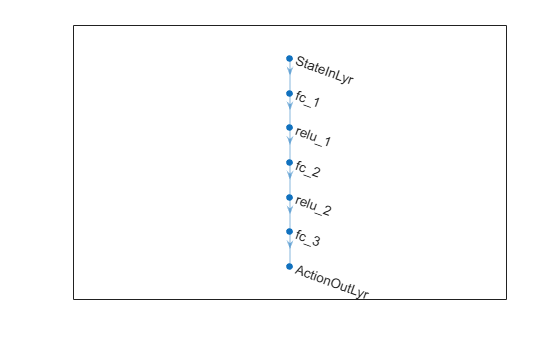
Define the network as an array of layer objects.

actorNet = [
    featureInputLayer(numObs, Name="StateInLyr")
    fullyConnectedLayer(64)
    reluLayer
    fullyConnectedLayer(32)
    reluLayer
    fullyConnectedLayer(numAct)
    tanhLayer(Name="ActionOutLyr")
    ];

Plot the actor network.

plot(layerGraph(actorNet));

Convert the network to a dlnetwork object.

actordlNet = dlnetwork(actorNet);

Display the number of parameters.

summary(actordlNet)

   Initialized: true

   Number of learnables: 2.7k

   Inputs:
      1   'StateInLyr'   8 features

Create the actor using rlContinuousDeterministicActor, passing the actor network and the environment specifications as input arguments.

actor = rlContinuousDeterministicActor(actordlNet,obsInfo,actInfo);

To create the TD3 agent, first specify the agent options using an rlTD3AgentOptions object. Alternatively, you can create the agent first, and then access its option object and modify all the options using dot notation.

The agent trains from an experience buffer of maximum capacity 2e6 by randomly selecting mini-batches of size 512. Use a discount factor of 0.995 to favor long-term rewards. TD3 agents maintain time-delayed copies of the actor and critics known as the target actor and critics. Configure the targets to update every 10 agent steps during training with a smoothing factor of 0.005.

Ts_agent = Ts;
agentOpts = rlTD3AgentOptions( ...
    SampleTime=Ts_agent, ...
    DiscountFactor=0.995, ...
    ExperienceBufferLength=2e6, ...
    MiniBatchSize=512, ...
    NumStepsToLookAhead=1, ...
    TargetSmoothFactor=0.005, ...
    TargetUpdateFrequency=10);

Specify training options for the critics and the actor using rlOptimizerOptions. For this example, set a learning rate of 1e-3 and 1e-4 for the actor and critics respectively.

% Critic optimizer options
for idx = 1:2
    agentOpts.CriticOptimizerOptions(idx).LearnRate = 1e-4;
    agentOpts.CriticOptimizerOptions(idx).GradientThreshold = 1;
end

% Actor optimizer options
agentOpts.ActorOptimizerOptions.LearnRate = 1e-3;
agentOpts.ActorOptimizerOptions.GradientThreshold = 1;
agentOpts.ActorOptimizerOptions.L2RegularizationFactor = 1e-3;

During training, the agent explores the action space using a Gaussian action noise model. Set the noise variance and decay rate using the ExplorationModel property. The noise variance decays at the rate of 2e-4, which favors exploration towards the beginning of training and exploitation in later stages. For more information on the noise model, see rlTD3AgentOptions.

agentOpts.ExplorationModel.Variance = 0.05;
agentOpts.ExplorationModel.VarianceDecayRate = 2e-4;
agentOpts.ExplorationModel.VarianceMin = 0.001;

The agent also uses a Gaussian action noise model for smoothing the target policy updates. Specify the variance and decay rate for this model using the TargetPolicySmoothModel property.

agentOpts.TargetPolicySmoothModel.Variance = 0.1;
agentOpts.TargetPolicySmoothModel.VarianceDecayRate = 1e-4;

Create the agent using the specified actor, critics, and options.

agent = rlTD3Agent(actor, [critic1,critic2], agentOpts);

Train Agent

To train the agent, first specify the training options using rlTrainingOptions. For this example, use the following options.

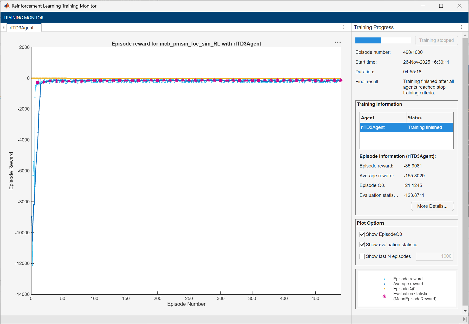
• Run each training for at most 1000 episodes, with each episode lasting at most ceil(T/Ts_agent) time steps.

• Stop training when the agent receives an average cumulative reward greater than -190 over 100 consecutive episodes. At this point, the agent can track the reference speeds.

T = 1.0;
maxepisodes = 1000;
maxsteps = ceil(T/Ts_agent); 
trainOpts = rlTrainingOptions(...
    MaxEpisodes=maxepisodes, ...
    MaxStepsPerEpisode=maxsteps, ...
    StopTrainingCriteria="AverageReward",...
    StopTrainingValue=-190,... 
    ScoreAveragingWindowLength=100);

Train the agent using the train function. Training this agent is a computationally intensive process that takes several minutes to complete. To save time while running this example, load a pretrained agent by setting doTraining to false. To train the agent yourself, set doTraining to true.

doTraining = false;
if doTraining
    trainResult = train(agent, env, trainOpts);
else
    load("rlPMSMAgent.mat","agent")
end

A snapshot of the training progress is shown in the following figure. You can expect different results due to randomness in the training process.

Simulate Agent

To validate the performance of the trained agent, simulate the model and view the closed-loop performance through the Speed Tracking Scope block.

sim(mdl);

You can also simulate the model at different reference speeds. Set the reference speed in the SpeedRef block to a different value between 0.2 and 1.0 per-unit and simulate the model again.

set_param("mcb_pmsm_foc_sim_RL/SpeedRef", "After", "0.6")
sim(mdl);

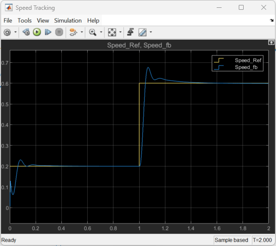
The following figure shows an example of closed-loop tracking performance. In this simulation, the reference speed steps through values of 695.4 rpm (0.2 per-unit) and 1738.5 rpm (0.5 pu). The PI and reinforcement learning controllers track the reference signal changes within 0.5 seconds.

Although the agent was trained to track the reference speed of 0.2 per-unit and not 0.5 per-unit, it was able to generalize well.

The following figure shows the corresponding current tracking performance. The agent was able to track the $\mathrm{id}$ and $\mathrm{iq}$ current references with steady-state error less than 2%.