Choose Trajectories for Manipulator Paths

This example provides an overview of the types of trajectories available in Robotics System Toolbox™. For manipulator motion, planning, and control applications, you must choose a trajectory for the robot to follow. There are three main sections of this example. The first section shows the types of trajectories that manipulators use, the second section demonstrates functions for generating trajectories, and the final section shows more tools for trajectory planning.

Trajectory Types for Manipulators

When using trajectories with manipulators, the goal is to provide a feasible result subject to certain constraints. For example, you often want a trajectory with smooth and continuous derivatives, such as one that does not require instantaneous velocity or acceleration. The trajectory may also be subject to position, velocity, or acceleration bounds. There are two general ways to use trajectories in the joint space and in the task space.

Joint-Space Trajectories

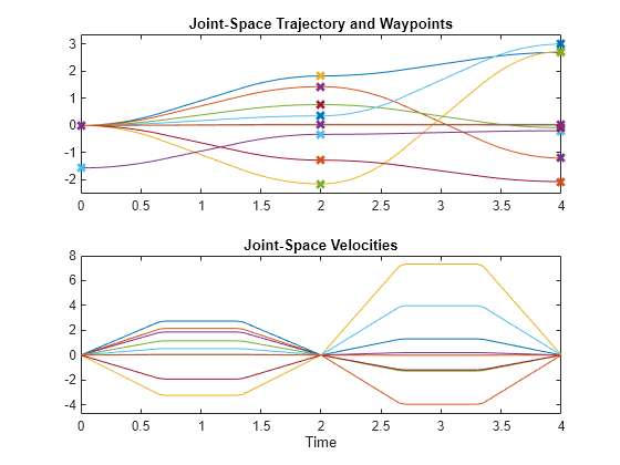
A joint-space trajectory typically contains a set of waypoints of multiple robot configurations connected using smooth motion. This example generates a trajectory using a trapezoidal velocity profile, which progressively speeds up each joint to a maximum velocity and slows it down as it approaches the next waypoint. For more information, see Trapezoidal Velocity Profile Trajectory.

Generate a trapezoidal velocity profile trajectory to connect waypoints for a Franka Emika Panda™ robot. First, define the time vector for the trajectories and load the robot model.

tpts = 0:4;
sampleRate = 20;
tvec = tpts(1):1/sampleRate:tpts(end);
numSamples = length(tvec);

robot = loadrobot("frankaEmikaPanda",DataFormat="column");

Define the joint-space trajectory. For this trajectory, the waypoints are the home configuration for the model and two random configurations.

rng default
frankaWaypoints = [robot.homeConfiguration robot.randomConfiguration robot.randomConfiguration];
frankaTimepoints = linspace(tvec(1),tvec(end),3);
[q,qd] = trapveltraj(frankaWaypoints,numSamples);

Visualize the robot executing the trajectory by iterating through the generated trajectory points q.

figure
set(gcf,"Visible","on");
rc = rateControl(sampleRate);
for i = 1:numSamples
    show(robot,q(:,i),FastUpdate=true,PreservePlot=false);
    waitfor(rc);
end

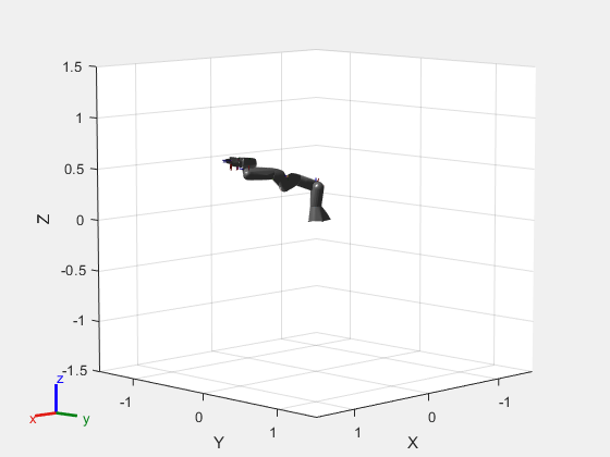
To examine the different joint positions and velocities, plot all the dimensions against time. Use the helperPlotJointSpaceTraj helper function to plot the joint-space trajectory and its waypoints.

helperPlotJointSpaceTraj("Joint-Space Trajectory and Waypoints", ...
    tvec,q,qd,frankaWaypoints,frankaTimepoints);

Task-Space Trajectories

A task-space trajectory contains waypoints that represent end-effector motion in 3-D space. Generate a minimum-jerk trajectory to connect waypoints in free space. The purpose of this trajectory profile is to create a smooth trajectory with minimal jerky motion. For more information, see Minimum-Jerk Trajectory. Then generate the joint configurations of the Franka Emika Panda robot using inverse kinematics.

First, create a set of waypoints, and then create the minimum-jerk trajectory using minjerkpolytraj.

frankaSpaceWaypoints = [0.5 0.25 0.25; 0.75 0 0.35; 0.5 -0.25 0.25; 0.5 0.25 0.25]';
frankaTimepoints = linspace(tvec(1),tvec(end),4);
[pos,vel] = minjerkpolytraj(frankaSpaceWaypoints,frankaTimepoints,numSamples);

Use the inverseKinematics function to create an inverse kinematics solver and solve for configurations that reach the desired end-effector positions over the trajectory.

rng(0) % Seed the RNG so the inverse kinematics solution is consistent
ik = inverseKinematics(RigidBodyTree=robot);
ik.SolverParameters.AllowRandomRestart = false;
q = zeros(9,numSamples);
weights = [0.2 0.2 0.2 1 1 1]; % Prioritize position over orientation
initialGuess = [0, 0, 0, -pi/2, 0, 0, 0, 0.01, 0.01]'; % Choose an initial guess within the robot joint limits
for i = 1:size(pos,2)
    targetPose = trvec2tform(pos(:,i)')*eul2tform([0, 0, pi]);
    q(:,i) = ik("panda_hand",targetPose,weights,initialGuess);
    initialGuess = q(:,i); % Use the last result as the next initial guess
end

Show the results using the robot model.

figure
set(gcf,"Visible","on")
show(robot);

rc = rateControl(sampleRate);
for i = 1:numSamples
    show(robot, q(:,i),FastUpdate=true,PreservePlot=false);
    waitfor(rc);
end

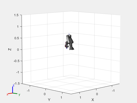
To examine the different joint positions and velocities, visualize these results by plotting all the dimensions against time. Use the helperPlotTaskSpaceTraj helper function to plot the task-space trajectory and its waypoints.

helperPlotTaskSpaceTraj("Task-Space Trajectory and Waypoints", ...
    tvec,pos,vel,frankaSpaceWaypoints,frankaTimepoints);

Compare Various Trajectory Profiles

Generate trajectories using different tools, and then compare them using both task- and joint-space visualization.

wpts = [0 45 15 90 45; 90 45 -45 15 90];
tpts = 0:(size(wpts,2)-1);

% Derived quantities.
sampleRate = 20;
tvec = tpts(1):1/sampleRate:tpts(end);
numSamples = length(tvec);

Minimum-Jerk Trajectory

The minjerkpolytraj function connects waypoints using a smooth, continuous motion. With the default boundary conditions, the trajectory has zero initial and final velocity, but passes through all intermediate waypoints with a continuous velocity.

Minimum-jerk trajectories are named as such because they minimize jerk, the third time-derivative of the motion, resulting in a smooth profile that is convenient for mechanical systems. The basic minimum-jerk trajectory is an analytical solution that hits the waypoints at the specified time points.

[q,qd,~,~,~,~,tvec] = minjerkpolytraj(wpts,tpts,numSamples);
helperPlotTaskSpaceTraj("Minimum-Jerk Trajectory",tvec,q,qd,wpts,tpts);

Trapezoidal Velocity Profile Trajectory

A trapezoidal velocity profile stops at each waypoint, and ensures smooth point-to-point motion. The profile name comes from the three phases of each segment that connects two waypoints:

• Acceleration from zero velocity to peak velocity

• Constant speed at the peak velocity

• Deceleration to zero velocity

This results in a velocity profile that is a trapezoid over each segment. Each segment is characterized by the end time, peak velocity, peak acceleration, and acceleration time parameters, but specifying any two is sufficient to fully define the motion. For more information, see trapveltraj.

You can use a basic trapezoidal profile when the goal is to connect a set of waypoints, stopping at each along the way. For example, this code connects waypoints using 1-second segments.

[q,qd,~,t] = trapveltraj(wpts,100);
helperPlotTaskSpaceTraj("Trapezoidal Profile, Max Velocity = 0.5",t,q,qd,wpts);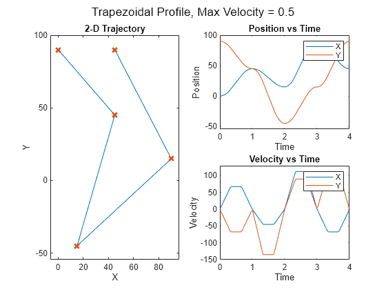

Trapezoidal profiles often seek to satisfy certain constraints, such as velocity or acceleration bounds. Because the trapezoidal profile is an exact specification, use a helper function to translate constraint bounds to exact profile specifications. The helperProfileForMaxVel helper function accepts velocity bounds. For more information on using the trapveltraj function to design velocity profiles, see the Design Trajectory with Velocity Limits Using Trapezoidal Velocity Profileexample.

[endTimes,peakVels] = helperProfileForMaxVel(wpts, 0.5);
[q,qd,~,t] = trapveltraj(wpts,100,EndTime=endTimes,PeakVelocity=peakVels);

% The time at which the waypoints are hit is the vector of cumulative sums
% of the end times
trapVelTrajTime = [0 cumsum(endTimes(1,:))];
helperPlotTaskSpaceTraj("Trapezoidal Profile, Max Velocity = 0.5",t,q,qd,wpts,trapVelTrajTime);

Cubic and Quintic Polynomial Trajectories

Some use cases can require a more general polynomial trajectory. The cubicpolytraj and quinticpolytraj functions are general tools for creating interpolating piecewise polynomials. Like the previous trajectory tools, they return position, velocity, and acceleration, as well as the piecewise polynomial object.

In the default case, these functions use zero-valued boundary conditions, resulting in trajectories that stop at every waypoint.

[q,qd] = cubicpolytraj(wpts,tpts,tvec);
helperPlotTaskSpaceTraj("Basic Cubic Polynomial",tvec,q,qd,wpts,tpts);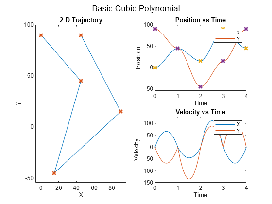

You can use these functions to design an interpolating polynomial with custom boundary behavior. For example, by using these functions together with other piecewise polynomial tools like spline, pchip, or makima, you can create smooth profiles with desirable motion at the waypoints.

This example code derives boundary conditions from one of the built-in piecewise polynomial functions in MATLAB®. Select a polynomial function to see how it affects the cubic polynomial velocity profile. The code uses a helper file to compute the velocity.

smoothPP = spline(tpts,wpts);
smoothVelPP = mkpp(smoothPP.breaks,robotics.core.internal.polyCoeffsDerivative(smoothPP.coefs),size(wpts,1));
smoothVelPoly = ppval(smoothVelPP,tpts);

Use the derived velocity as the boundary condition for the inner waypoints. Leave the outside boundary conditions as zero velocity to ensure the trajectory starts and ends at zero velocity.

boundaryVel = zeros(size(smoothVelPoly));
boundaryVel(:,2:end-1) = smoothVelPoly(:,2:end-1);
[q,qd] = cubicpolytraj(wpts,tpts,tvec,VelocityBoundaryCondition=boundaryVel);
helperPlotTaskSpaceTraj("Cubic Polynomial with Custom Velocity BCs",tvec,q,qd,wpts,tpts);

Using a quintic polynomial instead ensures a smooth velocity profile.

[q,qd] = quinticpolytraj(wpts,tpts,tvec,VelocityBoundaryCondition=boundaryVel);
helperPlotTaskSpaceTraj("Quintic Polynomial with Custom Velocity BCs",tvec,q,qd,wpts,tpts);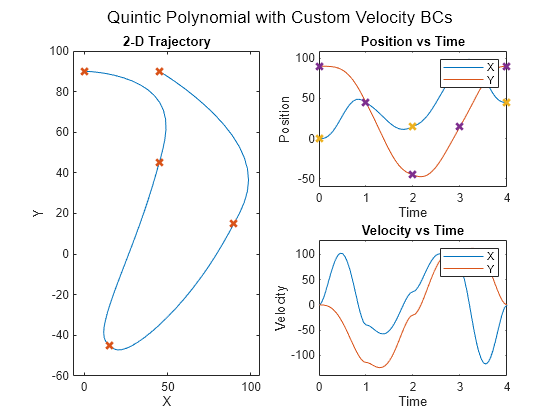

B-Spline Trajectory

A B-spline polynomial results in smooth, continuous motion, and is predominantly used for task-space applications. You can create this trajectory by using the bsplinepolytraj function. Unlike the other trajectories, which interpolate the waypoints that define them, a B-spline is defined by a set of control points. The resulting trajectory hits only the initial and final control points, but falls in the convex hull of the complete set of control points.

Apply the previously used waypoints as the control points.

[q,qd] = bsplinepolytraj(wpts,tpts([1 end]),tvec);
helperPlotTaskSpaceTraj("Non-interpolating B-spline",tvec,q,qd,wpts);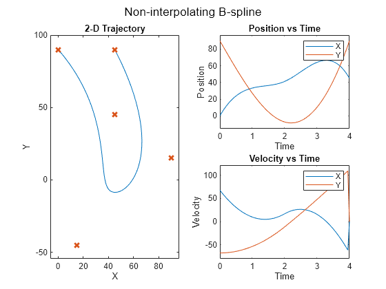

You can create an interpolating B-spline by deriving a new set of control points from the original waypoints, which the B-spline polynomial interpolates with the original waypoints. Like the standard B-spline, use this polynomial primarily for task-space applications.

Use the helperCreateControlPointsFromWaypoints helper function to derive the new control points.

cpts = helperCreateControlPointsFromWaypoints(wpts);
[q,qd] = bsplinepolytraj(cpts,tpts([1 end]),tvec);
helperPlotTaskSpaceTraj("Interpolating B-spline",tvec,q,qd,wpts);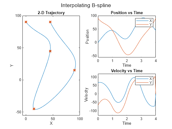

More Tools for Task-Space Trajectories

Some task-space applications benefit from computing not only the trajectories that interpolate positions, but also the full pose of the manipulator. In those cases, consider using the rottraj and transformtraj functions. The rottraj function creates a trajectory between two rotations, while the transformtraj function does the same for two 4-by-4 homogeneous transformation matrices. The functions output angular acceleration and velocity in addition to the position derivatives.

This example connects two poses, T1 and T2, which contain position and orientation data.

T1 = eul2tform([pi/4 0 pi/3]);
T2 = trvec2tform([5 -2 1]);
tInterval = [0 1];
tvec = 0:0.01:1;

Interpolate the two transformation matrices using transformtraj to create a trajectory of full, interpolated poses, represented as transformation matrices.

[tfInterp,v1,a1] = transformtraj(T1,T2,tInterval,tvec);

Plot the trajectory in 3-D space using plotTransforms. This function requires both the rotational data as a quaternion and the translational data from the interpolated transformation matrices trajectory. Use tform2quat to find the quaternion and tform2trvec to find the translational data from the trajectory.

figure
rotations = tform2quat(tfInterp);
translations = tform2trvec(tfInterp);
plotTransforms(translations,rotations)
title("Interpolated Transformation Trajectory")
xlabel("X")
ylabel("Y")
zlabel("Z")

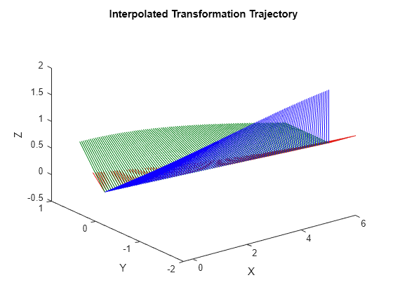
The 3-D plot shows that the rotations and motion are linear. Recall that feasible manipulator trajectories should be smooth and continuous. Because the interpolation is linear, the trajectory is not guaranteed to result in a smooth motion. This becomes clearer when you plot the position and velocities separately.

figure
tiles1 = tiledlayout(3,1)

tiles1 = 
  TiledChartLayout with properties:

    TileArrangement: 'fixed'
           GridSize: [3 1]
            Padding: 'loose'
        TileSpacing: 'loose'

  Use GET to show all properties

positions = reshape(tfInterp(1:3,4,:),3,size(tfInterp,3));
nexttile
plot(tvec,positions)
title("XYZ Position in Time")
ylim("padded")
nexttile
plot(tvec,v1(1:3,:))
title("Velocity in Time")
ylim("padded")
nexttile
plot(tvec,v1(4:6,:)); 
title("Angular Velocity in Time")
ylim("padded")

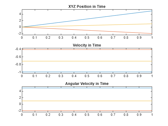
The velocities start and end at non-zero values, which is not a feasible trajectory for a manipulator, and would cause sudden and jerky motion.

You can use the TimeScaling name-value argument of transformtraj as a workaround. This argument defines the trajectory time using an intermediate parameterization, $\mathit{s}$, such that transformtraj is defined using $\mathit{s}\left(\mathit{t}\right)$ as time. In the default case used in this example, time scaling is uniform, so $\mathit{s}\left(\mathit{t}\right)=\mathit{t}$. The result is a linear motion between each pose. Instead, use time scaling defined by a minimum-jerk trajectory: $\mathit{s}\left(\mathit{t}\right)=$ minjerkpolytraj$\left(\mathit{t}\right)$.

Time scaling is a discrete set of values,$\left[\mathit{s};\frac{d}{\mathrm{d}\mathit{t}}\mathit{s};\frac{d^2}{\mathrm{d}{\mathit{t}}^2}\mathit{s}\right]$, which sample the function $\mathit{s}\left(\mathit{t}\right)$, defined on the interval $\mathit{s}=\left[0,1\right]$.

% The time scaling is a discrete set of values [s; ds/dt; d^2s/dt^2] that
% are sample the function s(t), defined on the interval s = [0,1]
[s,sd,sdd] = minjerkpolytraj([0 1],tInterval,numel(tvec));
[tfInterp,v1,a1] = transformtraj(T1,T2,tInterval,tvec,TimeScaling=[s; sd; sdd]);

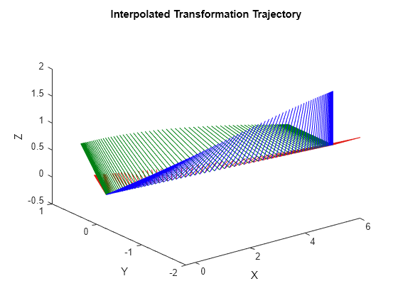
Plot the interpolated transformation trajectory again to compare against the previous plots.

figure
rotations = tform2quat(tfInterp);
translations = tform2trvec(tfInterp);
plotTransforms(translations,rotations)
title("Interpolated Transformation Trajectory")
xlabel("X")
ylabel("Y")
zlabel("Z")

figure
tiles2 = tiledlayout(3,1);
positions = reshape(tfInterp(1:3,4,:),3,size(tfInterp,3));
nexttile
plot(tvec,positions)
title("XYZ Position in Time")
nexttile
plot(tvec,v1(1:3,:))
title("Velocity in Time")
nexttile
plot(tvec,v1(4:6,:))
title("Angular Velocity in Time")

While the motion in space follows the same path, the second set of plots clarifies that the velocities are smooth and followable in time, resulting in a trajectory that is feasible for a manipulator or other mechanical system to follow.