bilinear

Bilinear transformation method for analog-to-digital filter conversion

Syntax

[zd,pd,kd] = bilinear(z,p,k,fs)

[numd,dend] = bilinear(num,den,fs)

[Ad,Bd,Cd,Dd] = bilinear(A,B,C,D,fs)

[___] = bilinear(___,fp)

Description

[zd,pd,kd] = bilinear(z,p,k,fs) converts the s-domain transfer function in pole-zero form specified by z, p, k and sample rate fs to a discrete equivalent.

[numd,dend] = bilinear(num,den,fs) converts the s-domain transfer function specified by numerator num and denominator den to a discrete equivalent.

[Ad,Bd,Cd,Dd] = bilinear(A,B,C,D,fs) converts the continuous-time state-space system in matrices A, B, C, and D to a discrete-time system.

[___] = bilinear(___,fp)uses parameter fp as "match" frequency to specify prewarping.

Examples

Bandpass IIR Filter Design Using Chebyshev Type I Analog Filter

Design the prototype for a 10th-order Chebyshev type I filter with 6 dB of ripple in the passband. Convert the prototype to state-space form.

[z,p,k] = cheb1ap(10,6);
[A,B,C,D] = zp2ss(z,p,k);  

Transform the prototype to a bandpass filter such that the equivalent digital filter has a passband with edges at 100 Hz and 500 Hz when sampled at a rate ${\mathit{f}}_{\mathit{s}}=2\mathrm{kHz}$. For the transformation, specify prewarped band edges ${\mathit{u}}_1$and ${\mathit{u}}_2$ in rad/s, a center frequency ${\mathit{W}}_{\mathit{o}}=\sqrt{{\mathit{u}}_1{\mathit{u}}_2}$, and a bandwidth ${\mathit{B}}_{\mathit{w}}={\mathit{u}}_2-{\mathit{u}}_1$.

fs = 2e3;

f1 = 100; u1 = 2*fs*tan(f1*(2*pi/fs)/2);
f2 = 500; u2 = 2*fs*tan(f2*(2*pi/fs)/2);

[At,Bt,Ct,Dt] = lp2bp(A,B,C,D,sqrt(u1*u2),u2-u1);

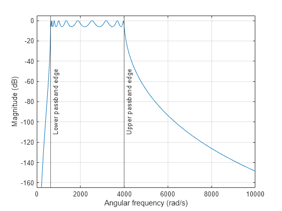
Compute the frequency response of the analog filter using freqs. Plot the magnitude response and the prewarped frequency band edges.

[b,a] = ss2tf(At,Bt,Ct,Dt);
[h,w] = freqs(b,a,2048);

plot(w,mag2db(abs(h)))
xline([u1 u2],"-",["Lower" "Upper"]+" passband edge", ...
    LabelVerticalAlignment="middle")

ylim([-165 5])
xlabel("Angular frequency (rad/s)")
ylabel("Magnitude (dB)")
grid

Use the bilinear function to create a digital bandpass filter with sample rate ${\mathit{f}}_{\mathit{s}}$.

[Ad,Bd,Cd,Dd] = bilinear(At,Bt,Ct,Dt,fs);

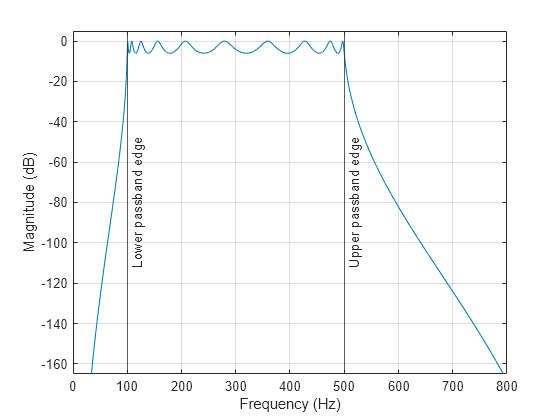
Convert the digital filter from state-space form to second-order sections and compute the frequency response using freqz. Plot the magnitude response and the passband edges.

[hd,fd] = freqz(ss2sos(Ad,Bd,Cd,Dd),2048,fs);

plot(fd,mag2db(abs(hd)))
xline([f1 f2],"-",["Lower" "Upper"]+" passband edge", ...
    LabelVerticalAlignment="middle")

ylim([-165 5])
xlabel("Frequency (Hz)")
ylabel("Magnitude (dB)")
grid

Discrete-Time Representation of Elliptic Filter

Design a 6th-order elliptic analog lowpass filter with 5 dB of ripple in the passband, a stopband attenuation of 90 dB, and a cutoff frequency ${\mathit{f}}_{\mathit{c}}=20\mathrm{Hz}$.

fc = 20;

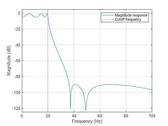
[z,p,k] = ellip(6,5,90,2*pi*fc,"s");

Visualize the magnitude response of the analog elliptic filter. Display the cutoff frequency.

[num,den] = zp2tf(z,p,k);
[h,w] = freqs(num,den,1024);

plot(w/(2*pi),mag2db(abs(h)))
xline(fc,Color=[0.8500 0.3250 0.0980])

axis([0 100 -125 5])
grid
legend(["Magnitude response" "Cutoff frequency"])
xlabel("Frequency (Hz)")
ylabel("Magnitude (dB)")

Use the bilinear function to transform the analog filter to a discrete-time IIR filter. Specify a sample rate ${\mathit{f}}_{\mathit{s}}=200\mathrm{Hz}$ and a prewarping match frequency ${\mathit{f}}_{\mathit{p}}=20\mathrm{Hz}$.

fs = 200;
fp = 20;

[zd,pd,kd] = bilinear(z,p,k,fs,fp);

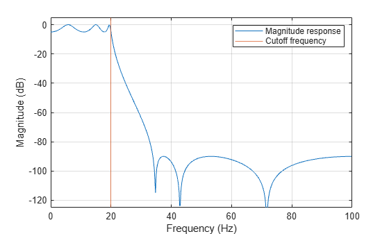
Visualize the magnitude response of the discrete-time filter. Display the cutoff frequency.

[hd,fd] = freqz(zp2sos(zd,pd,kd),[],fs);

plot(fd,mag2db(abs(hd)))
xline(fc,Color=[0.8500 0.3250 0.0980])

axis([0 100 -125 5])
grid
legend(["Magnitude response" "Cutoff frequency"])
xlabel("Frequency (Hz)")
ylabel("Magnitude (dB)")

Input Arguments

z, p, k — Analog-domain zeros, poles, and gain

column vectors, scalar

Zeros, poles, and gain of the s-domain transfer function, specified as two column vectors and a scalar.

fs — Sample rate

positive scalar

Sample rate, specified as a positive scalar.

num, den — Analog-domain numerator and denominator coefficients

row vectors

Numerator and denominator coefficients of the analog transfer function, specified as row vectors.

A, B, C, D — Analog-domain state-space matrices

matrices

State-space representation in the s-domain, specified as matrices. If the system has p inputs and q outputs and is described by n state variables, then A is n-by-n, B is n-by-p, C is q-by-n, and D is q-by-p.

Data Types: single | double

fp — Match frequency

positive scalar

Match frequency, specified as a positive scalar.

Output Arguments

zd, pd, kd — Digital-domain zeros, poles, and gain

column vectors, scalar

Zeros, poles, and gain of the z-domain transfer function, returned as column vectors and a scalar.

numd, dend — Digital-domain numerator and denominator coefficients

row vectors

Numerator and denominator coefficients of the digital transfer function, returned as row vectors.

Ad, Bd, Cd, Dd — Digital-domain state-space matrices

matrices

State-space representation in the z-domain, returned as matrices. If the system is described by n state variables and has q outputs, then Ad is n-by-n, Bd is n-by-1, Cd is q-by-n, and Dd is q-by-1.

Data Types: single | double

Algorithms

The bilinear transformation is a mathematical mapping of variables. In digital filtering, it is a standard method of mapping the s or analog plane into the z or digital plane. It transforms analog filters, designed using classical filter design techniques, into their discrete equivalents.

The bilinear transformation maps the s-plane into the z-plane by

$${H(z)=H(s)|}_{s=2f_s\frac{z-1}{z+1}}.$$

This transformation maps the jΩ axis (from Ω = –∞ to +∞) repeatedly around the unit circle (e^jω, from ω = –π to π) by

$$\omega =2{\tan }^{-1}\left(\frac{\Omega }{2f_s}\right).$$

bilinear can accept an optional parameter Fp that specifies prewarping. fp, in hertz, indicates a "match" frequency for which the frequency responses before and after mapping match exactly. In prewarped mode, the bilinear transformation maps the s-plane into the z-plane with

$${H(z)=H(s)|}_{s=\frac{2\pi f_p}{\tan \left(\pi \frac{f_p}{f_s}\right)}\frac{z-1}{z+1}}.$$

With the prewarping option, bilinear maps the jΩ axis (from Ω = –∞ to +∞) repeatedly around the unit circle (e^jω, from ω = –π to π) by

$$\omega =2{\tan }^{-1}\left(\frac{\Omega \tan \left(\pi \frac{f_p}{f_s}\right)}{2\pi f_p}\right).$$

In prewarped mode, bilinear matches the frequency 2πf_p (in radians per second) in the s-plane to the normalized frequency 2πf_p/f_s (in radians per second) in the z-plane.

The bilinear function works with three different linear system representations: zero-pole-gain, transfer function, and state-space form.

bilinear uses one of two algorithms depending on the format of the input linear system you supply. One algorithm works on the zero-pole-gain format and the other on the state-space format. For transfer function representations, bilinear converts to state-space form, performs the transformation, and converts the resulting state-space system back to transfer function form.

Zero-Pole-Gain Algorithm

For a system in zero-pole-gain form, bilinear performs four steps:

1. If fp is present, it prewarps:

   fp = 2*pi*fp;
   fs = fp/tan(fp/fs/2)
   

   otherwise, fs = 2*fs.

2. It strips any zeros at ±∞ using

   z = z(finite(z));
   

3. It transforms the zeros, poles, and gain using

   pd = (1+p/fs)./(1-p/fs);    % Do bilinear transformation
   zd = (1+z/fs)./(1-z/fs);
   kd = real(k*prod(fs-z)./prod(fs-p));
   

4. It adds extra zeros at -1 so the resulting system has equivalent numerator and denominator order.

State-Space Algorithm

An analog system in state space form is given by

$$\begin{array}{l}\dot{x}=Ax+Bu\\ y=Cx+Du\end{array}$$

. This system is converted to the discrete form using state-space equations as follows:

$$\begin{array}{l}x[n+1]=A_{d}x[n]+B_{d}u[n],\\ y[n]=C_{d}x[n]+D_{d}u[n].\end{array}$$

To convert an analog system in state-space form, bilinear performs two steps:

1. If fp is present, let

   $$\lambda =\frac{\pi f_p}{\tan (\pi f_p/f_s)}.$$

   If fp is not present, let λ=fs.

2. Compute Ad, Bd, Cd, and Dd in terms of A, B, C, and D using

   $$\begin{array}{l}{A}_d={(}^I(I+A\frac{1}{2\lambda }),\\ B_d=\frac{1}{\sqrt{\lambda }}{(}^{I}B,\\ C_d=\frac{1}{\sqrt{\lambda }}C{(}^I,\\ D_d=\frac{1}{2\lambda }C{(}^{I}B+D.\end{array}$$

Transfer Function

For a system in transfer function form, bilinear converts an s-domain transfer function given by num and den to a discrete equivalent. Row vectors num and den specify the coefficients of the numerator and denominator, respectively, in descending powers of s. Let B(s) be the numerator polynomial and A(s) be the denominator polynomial. The transfer function is:

$$\frac{B(s)}{A(s)}=\frac{B(1)s^n+\cdots +B(n)s+B(n+1)}{A(1)s^m+\cdots +A(m)s+A(m+1)}$$

fs is the sample rate in hertz. bilinear returns the discrete equivalent in row vectors numd and dend in descending powers of z (ascending powers of z^–1). fp is the optional match frequency, in hertz, for prewarping.

References

[1] Oppenheim, Alan V., and Ronald W. Schafer, with John R. Buck. Discrete-Time Signal Processing. Upper Saddle River, NJ: Prentice Hall, 1999.

[2] Parks, Thomas W., and C. Sidney Burrus. Digital Filter Design. New York: John Wiley & Sons, 1987.

Extended Capabilities

C/C++ Code Generation
Generate C and C++ code using MATLAB® Coder™.

Version History

Introduced before R2006a

References

[1] Al-Saggaf, Ubaid M., and Gene F. Franklin. “Model Reduction via Balanced Realizations: An Extension and Frequency Weighting Techniques.” IEEE Transactions on Automatic Control 33, no. 7 (July 1988): 687–92. https://doi.org/10.1109/9.1280.