firpm
Parks-McClellan optimal FIR filter design
Syntax
Description
Examples
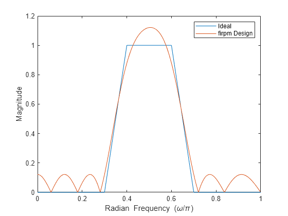
Use the Parks-McClellan algorithm to design an FIR bandpass filter of order 17. Specify normalized stopband frequencies of and rad/sample and normalized passband frequencies of and rad/sample. Plot the ideal and actual magnitude responses.
f = [0 0.3 0.4 0.6 0.7 1];
a = [0 0 1 1 0 0];
b = firpm(17,f,a);

[h,w] = freqz(b,1,512);
plot(f,a,w/pi,abs(h))
legend('Ideal','firpm Design')
xlabel 'Radian Frequency (\omega/\pi)', ylabel 'Magnitude'
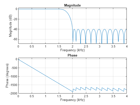
Design a lowpass filter with a 1500 Hz passband cutoff frequency and 2000 Hz stopband cutoff frequency. Specify a sampling frequency of 8000 Hz. Require a maximum stopband amplitude of 0.01 and a maximum passband error (ripple) of 0.001. Obtain the required filter order, normalized frequency band edges, frequency band amplitudes, and weights using firpmord.
[n,fo,ao,w] = firpmord([1500 2000],[1 0],[0.001 0.01],8000);
b = firpm(n,fo,ao,w);
freqz(b,1,[],8000)
Use the Parks-McClellan algorithm to create a 50th-order equiripple FIR bandpass filter to be used with signals sampled at 1 kHz.
N = 50;
Fs = 1e3;
Specify that the passband spans the frequencies between 200 Hz and 300 Hz and that the transition region on either side of the passband has a width of 50 Hz.
Fstop1 = 150;
Fpass1 = 200;
Fpass2 = 300;
Fstop2 = 350;
Design the filter so that the optimization fit weights the low-frequency stopband with a weight of 3, the passband with a weight of 1, and the high-frequency stopband with a weight of 100. Display the magnitude response of the filter.
Wstop1 = 3;
Wpass = 1;
Wstop2 = 100;

b = firpm(N,[0 Fstop1 Fpass1 Fpass2 Fstop2 Fs/2]/(Fs/2), ...
    [0 0 1 1 0 0],[Wstop1 Wpass Wstop2]);

freqz(b,1)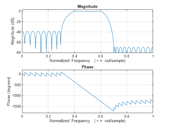
Input Arguments
Output Arguments
More About
Tips
If your filter design fails to converge, the filter design might not be correct. Verify the design by checking the frequency response.
If your filter design fails to converge and the resulting filter design is not correct, attempt one or more of the following:
Increase the filter order.
Relax the filter design by reducing the attenuation in the stopbands and/or broadening the transition regions.
Algorithms
firpm designs a linear-phase FIR filter using the Parks-McClellan
algorithm [2]. The Parks-McClellan algorithm uses the Remez exchange algorithm and
Chebyshev approximation theory to design filters with an optimal fit between the desired
and actual frequency responses. The filters are optimal in the sense that the maximum
error between the desired frequency response and the actual frequency response is
minimized. Filters designed this way exhibit an equiripple behavior in their frequency
responses and are sometimes called equiripple filters. firpm exhibits
discontinuities at the head and tail of its impulse response due to this equiripple
nature.
These are type I (n odd) and type II (n even)
linear-phase filters. Vectors f and a specify the
frequency-amplitude characteristics of the filter:
fis a vector of pairs of frequency points, specified in the range between 0 and 1, where 1 corresponds to the Nyquist frequency. The frequencies must be in increasing order.ais a vector containing the desired amplitude at the points specified inf.The desired amplitude function at frequencies between pairs of points (f(k), f(k+1)) for k odd is the line segment connecting the points (f(k), a(k)) and (f(k+1), a(k+1)).
The desired amplitude function at frequencies between pairs of points (f(k), f(k+1)) for k even is unspecified. These are transition or "don’t care" regions.
fandaare the same length. This length must be an even number.
The figure below illustrates the relationship between the f and
a vectors in defining a desired amplitude response.

firpm always uses an even filter order for configurations with even
symmetry and a nonzero passband at the Nyquist frequency. The reason for the even filter
order is that for impulse responses exhibiting even symmetry and odd orders, the
frequency response at the Nyquist frequency is necessarily 0. If you specify an
odd-valued n, firpm increments it by 1.
firpm designs type I, II, III, and IV linear-phase filters. Type I
and type II are the defaults for n even and n odd,
respectively, while type III (n even) and type IV
(n odd) are specified with 'hilbert' or
'differentiator', respectively, using the
ftype argument. The different types of filters have different
symmetries and certain constraints on their frequency responses. (See [3] for more details.)
| Linear Phase Filter Type | Filter Order | Symmetry of Coefficients | Response H(f),
f = 0 | Response H(f),
f = 1
(Nyquist) |
|---|---|---|---|---|
Type I | Even | even: | No restriction | No restriction |
Type II | Odd | even: | No restriction | H(1)
|
Type III | Even | odd: | H(0) | H(1) |
| Type IV | Odd | odd: | H(0) | No restriction |
You can also use firpm to write a function that defines the desired
frequency response. For more information, see User-Defined Frequency Response Functions.
References
[1] Digital Signal Processing Committee of the IEEE Acoustics, Speech, and Signal Processing Society, eds. Selected Papers in Digital Signal Processing. Vol. II. New York: IEEE Press, 1976.
[2] Digital Signal Processing Committee of the IEEE Acoustics, Speech, and Signal Processing Society, eds. Programs for Digital Signal Processing. New York: IEEE Press, 1979, algorithm 5.1.
[3] Oppenheim, Alan V., Ronald W. Schafer, and John R. Buck. Discrete-Time Signal Processing. Upper Saddle River, NJ: Prentice Hall, 1999, p. 486.
[4] Parks, Thomas W., and C. Sidney Burrus. Digital Filter Design. New York: John Wiley & Sons, 1987, p. 83.
[5] Rabiner, Lawrence R., James H. McClellan, and Thomas W. Parks. "FIR Digital Filter Design Techniques Using Weighted Chebyshev Approximation." Proceedings of the IEEE®. Vol. 63, Number 4, 1975, pp. 595–610.
Extended Capabilities
Version History
Introduced before R2006a