freqs
Frequency response of analog filters
Description
freqs(___) with no output arguments plots the magnitude
and phase responses as functions of angular frequency in the current figure window. You can
use this syntax with either of the previous input syntaxes.
Examples
Find and graph the frequency response of the transfer function
a = [1 0.4 1];
b = [0.2 0.3 1];
w = logspace(-1,1);

h = freqs(b,a,w);
mag = abs(h);
phase = angle(h);
phasedeg = phase*180/pi;

subplot(2,1,1)
loglog(w,mag)
grid on
xlabel('Frequency (rad/s)')
ylabel('Magnitude')

subplot(2,1,2)
semilogx(w,phasedeg)
grid on
xlabel('Frequency (rad/s)')
ylabel('Phase (degrees)')
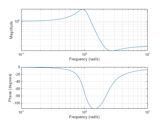
You can also generate the plots by calling freqs with no output arguments.
figure
freqs(b,a,w)

Design a fifth-order analog Butterworth lowpass filter with a cutoff frequency of 2 GHz. Multiply by to convert the frequency to radians per second. Compute the frequency response of the filter at 4096 points.
n = 5;
wn = 2*pi*2e9;
w = 2*pi*1e9*logspace(-2,1,4096)';

[zb,pb,kb] = butter(n,wn,"s");
[bb,ab] = zp2tf(zb,pb,kb);
[hb,wb] = freqs(bb,ab,w);
gdb = -diff(unwrap(angle(hb)))./diff(wb);
Design a fifth-order Chebyshev Type I filter with a passband edge frequency of 2 GHz and 3 dB of passband ripple. Compute its frequency response.
wp = wn;

[z1,p1,k1] = cheby1(n,3,wp,"s");
[b1,a1] = zp2tf(z1,p1,k1);
[h1,w1] = freqs(b1,a1,w);
gd1 = -diff(unwrap(angle(h1)))./diff(w1);
Design a fifth-order Chebyshev Type II filter with a stopband edge frequency of 2.5 GHz and 30 dB of stopband attenuation. Compute its frequency response.
ws = 2*pi*2.5e9;

[z2,p2,k2] = cheby2(n,30,ws,"s");
[b2,a2] = zp2tf(z2,p2,k2);
[h2,w2] = freqs(b2,a2,w);
gd2 = -diff(unwrap(angle(h2)))./diff(w2);
Design a fifth-order elliptic filter with the same passband and stopband edge frequencies, 3 dB of passband ripple, and 30 dB of stopband attenuation. Compute its frequency response.
[ze,pe,ke] = ellip(n,3,30,wp,"s");
[be,ae] = zp2tf(ze,pe,ke);
[he,we] = freqs(be,ae,w);
gde = -diff(unwrap(angle(he)))./diff(we);
Design a fifth-order Bessel filter with the same edge frequency. Compute its frequency response.
[zf,pf,kf] = besself(n,wn);
[bf,af] = zp2tf(zf,pf,kf);
[hf,wf] = freqs(bf,af,w);
gdf = -diff(unwrap(angle(hf)))./diff(wf);
Plot the attenuation in decibels. Express the frequency in gigahertz. Compare the filters.
fGHz = [wb w1 w2 we wf]/(2e9*pi);
plot(fGHz,mag2db(abs([hb h1 h2 he hf])))
axis([0 5 -45 5])
grid on
xlabel("Frequency (GHz)")
ylabel("Attenuation (dB)")
legend(["butter" "cheby1" "cheby2" "ellip" "besself"], ...
    Location="southwest")

The Butterworth and Chebyshev Type II filters have flat passbands and wide transition bands. The Chebyshev Type I and elliptic filters roll off faster but have passband ripple. The frequency input to the Chebyshev Type II design function sets the beginning of the stopband rather than the end of the passband. Elliptic filters offer steeper rolloff characteristics than Butterworth and Chebyshev filters, but they are equiripple in both the passband and the stopband. Of these four classical filter types, elliptic filters usually meet a given set of filter performance specifications with the lowest filter order.
Plot the group delay in samples. Express the frequency in gigahertz and the group delay in nanoseconds. Compare the filters. The Bessel filter has approximately constant group delay along the passband.
gdns = [gdb gd1 gd2 gde gdf]*1e9;
gdns(gdns<0) = NaN;
loglog(fGHz(2:end,:),gdns)
grid on
xlabel("Frequency (GHz)")
ylabel("Group delay (ns)")
legend(["butter" "cheby1" "cheby2" "ellip" "besself"], ...
    Location="southwest")

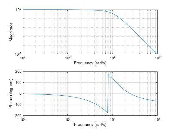
Design a 5th-order analog lowpass Bessel filter with an approximately constant group delay up to rad/s. Plot the frequency response of the filter using freqs.
[b,a] = besself(5,10000);   % Bessel analog filter design
freqs(b,a)                  % Plot frequency response
Input Arguments
Output Arguments
Algorithms
freqs returns the complex frequency response of an analog filter
specified by b and a. The function evaluates the
ratio of Laplace transform polynomials
along the imaginary axis at the frequency points s = jω:
s = 1j*w;
h = polyval(b,s)./polyval(a,s);
Version History
Introduced before R2006a